

|
|
Calculating forces at focal adhesions
Reconstructing point forces at focal adhesions
This website provides technical information on a procedure which we developed in order to calculate localized (point) forces at focal adhesions from elastic substrate data. Experimental and theoretical issues related to our procedure as well as results obtained can be found in the following publications:- N. Q. Balaban, U. S. Schwarz, D. Riveline, P. Goichberg, G. Tzur, I. Sabanay, D. Mahalu, S. Safran, A. Bershadsky, L. Addadi and B. Geiger, Force and focal adhesion assembly: a close relationship studied using elastic micro-patterned substrates, Nat. Cell Biol. 3: 466-472 (2001) (abstract, PDF)
- U. S. Schwarz, N. Q. Balaban, D. Riveline, A. Bershadsky, B. Geiger, S. A. Safran, Calculation of forces at focal adhesions from elastic substrate data: the effect of localized force and the need for regularization, Biophys. J. 83: 1380-1394 (2002) (abstract, PDF)
- U. S. Schwarz, N. Q. Balaban, D. Riveline, L. Addadi, A. Bershadsky, S. A. Safran, B. Geiger, Measurement of cellular forces at focal adhesions using elastic micro-patterned substrates, Mat. Sci. Eng. C 23: 387-394 (2003) (abstract, PDF)
- B. Sabass, M. L. Gardel, C. Waterman and U. S. Schwarz. High resolution traction force microscopy based on experimental and computational advances. Biophys. J., 94:207-220, 2008. (abstract, doi:10.1529/biophysj.107.113670, PDF)
General remarks
Measuring cellular forces on the level of single cell-matrix contacts is a difficult task for several reasons, and there is no single techniques yet which avoids all potential problems. Here we list some of the issues involved:- All force sensors will be some kind of spring, whose spring constant has to be matched to the cellular force. There are several techniques which have been employed over the last years to measure pN-forces on the level of single molecules (including atomic force microscopy and optical tweezers), but all of them are too weak to measure the nN-forces which act at single cell-matrix contacts. Prestressed thin elastic films turned out to allow quantitative analysis of the forces exerted by keratocytes, but were too weak for fibroblast traction, for which one has to use thick elastic films.
- Typically a cell adheres simultaneously at hundreds or thousands of contacts. Local force probes like cantilevers micromachined in silicon wafers have been shown to work for single contacts, but in order to monitor all contacts, one needs many of those. Microfabricated arrays of elastic needles can provide sensor densities of down to one per square micron, but restrict contacts to form on the needle tips.
- All techniques used up to now are restricted to measure force only in certain directions: eg a cantilever device or microneedle can only measure force perpendicular to the lever arm, and elastic substrates have been used only to measure forces tangentially to the plane of the substrate.
- Depending on cell type, cells react very sensitively to chemical, mechanical and topographical features of their environment. Any new experimental technique introduced has to be proven not to disturb the normal functioning of the cell. In this vein, the bulky features of cantilevers and microneedles, the small rigidity of elastic substrates and the topographic patterning of elastic substrates might turn out to be problematic.
- The ideal force probe would allow for direct reading of the force value. For example, a cantilever or microneedle with a known spring constant allows direct measurement of force by reading of displacement. In contrast, elastic substrates need calculations to reconstruct the force pattern from the displacement data.
Recently, we adapted the elastic substrate technique for the special purpose of measuring forces at single focal adhesions. Our technique combines three elements:
- The use of micro-patterned elastic substrates allows immediate visualization of cell traction and easy extraction of displacement. Thus it is an attractive alternative to the use of marker beads embedded in the substrate. In our work, we used both topographic and fluorescent patterning, which can be evaluated by image analysis of phase contrast and fluroescence pictures, respectively.
- The use of GFP-vinculin allows to extract position, size and orientation of the focal adhesions from fluorescence pictures.
- Numerical solution of the (ill-posed) inverse problem of linear elasticity allows to estimate the force pattern from the displacement data. In contrast to earlier work, we assume point forces at focal adhesions, whose positions are known from the fluorescence data. This procedure has two advantages: the resulting numerics is much faster than for the case of a continuous force field underneath the cell body, and the calculated forces can be easily correlated with other features of the focal adhesions (namely size and orientation).
Data files
The input and output data of our numerics consist of several ASCII datafiles:- lines.dat: displacement data extracted by image processing of phase contrast or fluorescence pictures showing the patterned substrate. Our micropattern consisted of a cubic array of small dots, whose positions had to be determined with and without traction. In order to get the reference image, cells were trypsinized, but the reference points can also be constructed by extrapolating the undistorted coordinate system from the far field image of the image under traction. In order to extract the dot positions, we used the water algorithm (E. Zamir et al., J. Cell Sci. 1999), which fits an ellipse to each dot. The ellipse midpoint is then identified with the dot position. Each line of the file contains data for one dot displacement in the form x1 y1 x2 y2.
- focals.dat: focal adhesion data extracted by image processing from fluorescence pictures. Again the water algorithm has been used to find focal adhesion positions (moreoever it gives focal adhesion size and orientation, which were later used for correlation studies). Each line contains data for the position of one focal adhesion in the form x y.
- newlines.dat: in principle the same data as in lines.dat, but cleaned by some data whose use is not reasonable for some reason. For example, since our approach uses point forces at focal adhesions (ie Green functions which diverge like 1/r), displacement data should not be used if it is closer to the focal adhesion midpoint than the typical lateral extension of focal adhesions. In our paper in BPJ, we showed that with this precaution, the point forces described by Green functions are good approximations in the sense of a force multipolar expansion to the distributed forces acting at focal adhesions.
- forces.dat: this is the desired output of our calculation: for each line in newfocals.dat, forces.dat gives the estimate point force in the form fx fy.
Numerical procedure
As explained in our paper in BPJ, the inverse problem of linear elasticity (calculating force from displacement) is ill-posed and the calculated force pattern will be unreliable if not regularized by some appropriate side constraint. The simplest solution to this problem is use of Tikhonov regularization, which is a well established technique covered in many textbooks. For our work, we have used a freely available package of Matlab routines to do this job. The author of these routines is Prof. Per Christian Hansen, who has turned his PhD-thesis on this subject into a book (P. C. Hansen, Rank-Deficient and Discrete Ill-Posed Problems: Numerical Aspects of Linear Inversion, SIAM, Philadelphia, 1998). His accompaying software Regularization Tools can be downloaded from his webpage and is also available in the NumerAlgo directory at Netlib. If you want to use our program, you should first download our routines and extract them to some directory. Then you should download Prof. Hansen's software and unpack it into a subdirectory with the name Hansen. If you then start up Matlab for the directory with our routines, there should be the data files lines.dat and focals.dat included in our software bundle to work with. These two files represent artificial data which we generated in order to check how our technique is working.First you should use the routine data.m, which converts the file lines.dat into newlines.dat. It also produces the following plot:
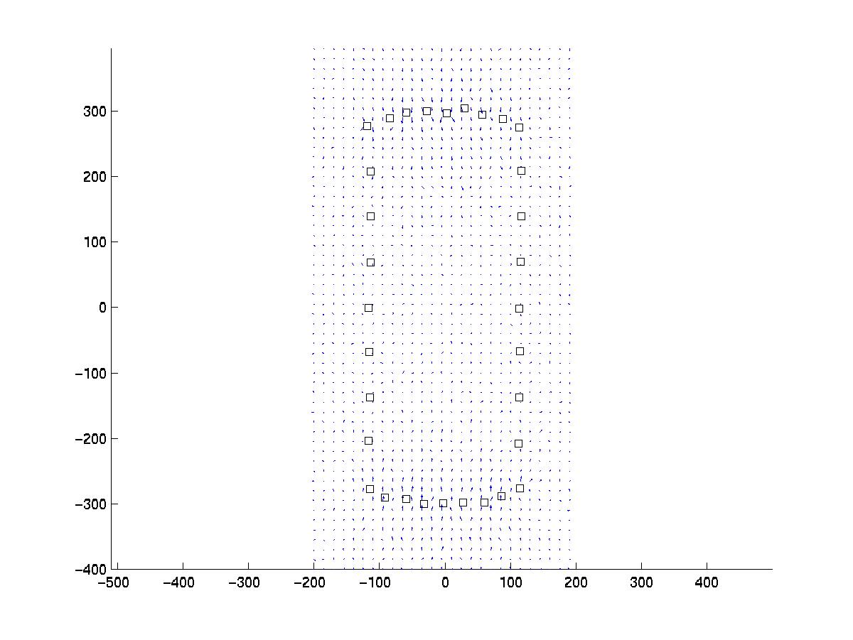
Our artificial pattern of point force positions (squares) can be imagined to be a set of focal adhesions distributed along the rim of a polarized cell. The resulting displacement has been calculated on a cubic array and some noise has been added with a standard deviation of sigma = 1 pixel, which in an experiment has to be estimated from the data, eg by analyzing images without cell traction.
Next you can use the routine inverse.m to estimate the original force pattern from this data. The routine first reads in the data newlines.dat and focals.dat and plot the same picture as above. It then calculates the matrix and its singular value decomposition for the linear mapping between force and displacement from the Green function for an isotropic elastic halfspace. This might take a while, depending on the number of displacements and focals. Once this is done, the system of linear equations can be quickly inverted for different values of the regularization parameter. The program then plots the residual norm R as a function of regularization parameter lambda (blue line with sigmoidal shape):
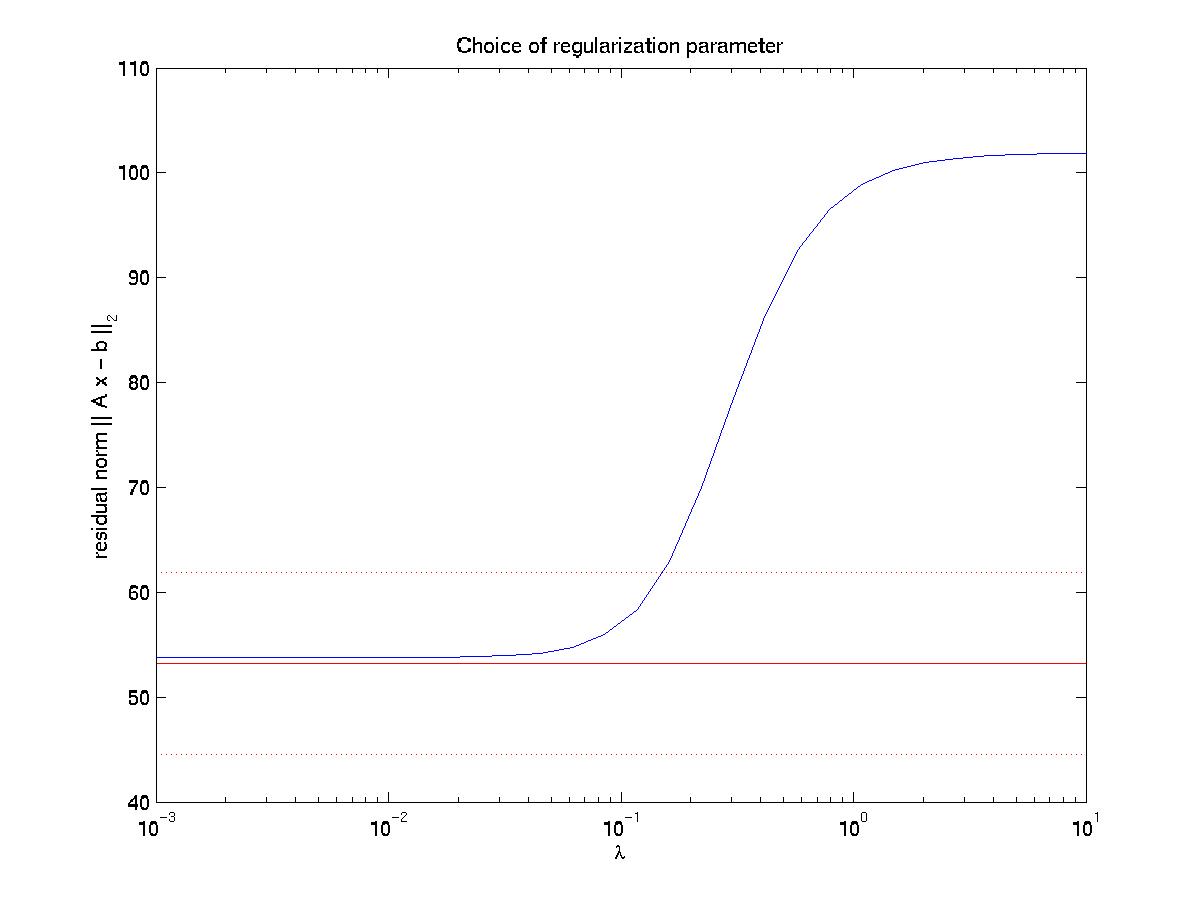
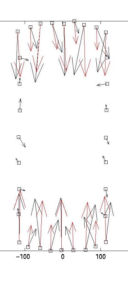
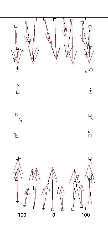
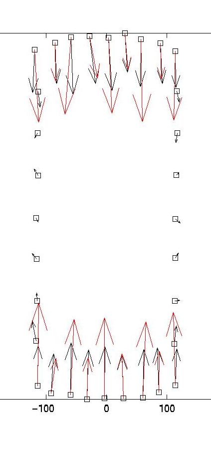
The solid and dotted red lines represent the chi-squared estimate for the confidence interval for R, based on the value for sigma, the displacement noise level. For most noise realizations, the solid red line will cut the blue one, indicating the optimal value for lambda. In the case shown here, it just fails to do so, thus one has to choose a value which is closer to the upper end of the interval. This is a weakness of the chi-square criterion. Another simple criterion would be to determine the value of lambda at which the blue curve starts to rise significantly from the plateau, eg as evidenced by a L-curve plot (not shown here) or by visual inspection. In our case, this suggests a value around lambda = 0.03. Giving a lambda value to the program yields a plot for the corresponding force estimate. At the same time, the force estimate is saved as forces.dat. The program then loops and asks for a different value of lambda. Giving lambda = 0 terminates the loop. Here we also show force reconstructions for lambda = 0.01 and 0.1, which bracket the optimal estimate for lambda = 0.03. The red arrows are the original forces, which we know since we use an artificial force pattern:
 |
 |
 |
|
|
|
|
On the left, we see that lambda values which are too small result in force details which are artifacts resulting from the noise in the displacement data (eg original forces had only small x-components and vanish at the sides). On the right, we see that lambda values which are too large lead to small forces with little spatial resolution (eg the magnitude of the original forces oscillates). As explained in our paper in BPJ, these calculations are estimates and a perfect reconstruction of the original force pattern cannot be expected. Yet for the optimal lambda value, the agreement between original and reconstructed forces is certainly not bad. In particular, the spatial resolution between the different contacts is reasonable. If one uses our program on experimental data, one should of course comment out the few lines related to the original force data, which only exists for artificial force patterns like the one provided with our software.
Finally one has to calibrate the data. The Green function used in our software is specified for the incompressible case of Poisson ratio = 0.5. Moreover one has to know the Young modulus E and the microscope magnification. Eg for a 100x magnification, 1 pixel = 0.13328 micron. In order to get the force scale right, one has to use the following formula:
Eg for E = 10 kPa, the factor 10*(0.133)^2 = 0.177 arises: one pixel correspond to 0.177 nN.
| This software is free, but if you use it for your own work, you should acknowledge its use and cite our published work (i.e. the papers in Nat. Cell Biol. and Biophys. J.). In particular, you should read the paper in Biophys. J. to understand what the routines are about. For comments and questions, please address Ulrich.Schwarz@bioquant.uni-heidelberg.de. |
Last modified Mon May 4 13:25:57 CEST 2009
by USS.
Back to home page Ulrich Schwarz.