
Quantum field theory 1, lecture 11
6 Non-relativistic bosons
6.1 Functional integral for spinless atoms
From relativistic to non-relativistic scalar fields. In this section we go from a relativistic quantum field theory back to non-relativistic physics but in a quantum field theoretic formalism. This non-relativistic QFT is in the few-body limit equivalent to quantum mechanics for a few particles but also has interesting applications to condensed matter physics (many body quantum theory) and it is interesting conceptually. We start from the action of a complex, relativistic scalar field in Minkowski space \begin{equation*} S=\int dt d^3x \left \{-\partial _\mu \phi ^*\partial ^\mu \phi - m^2\phi ^*\phi - \frac{\lambda }{2}(\phi ^*\phi )^2\right \}. \end{equation*} The quadratic part can be written in Fourier space with (\(px = -p^0x^0 + \vec{p}\vec{x}\)), \begin{equation*} \phi (x) = \int \frac{d^4 p}{(2\pi )^4} e^{ipx} \phi (p), \quad \quad \quad \phi ^*(x) = \int \frac{d^4 p}{(2\pi )^4} e^{-ipx} \phi ^*(p), \end{equation*} as \begin{equation*} \begin{split} S_2 = & -\int \frac{d^4 p}{(2\pi )^4}\left \{\phi ^*(p)\left [-(p^0)^2+\vec{p}^2+m^2\right ]\phi (p)\right \} \\ = & -\int \frac{d^4 p}{(2\pi )^4}\left \{\phi ^*(p)\left [-\left (p^0-\sqrt{\vec{p}^2+m^2}\right )\left (p^0+\sqrt{\vec{p}^2+m^2} \right )\right ]\phi (p)\right \}. \end{split} \end{equation*}
Two zero crossings. One observes that the so-called inverse propagator has two zero-crossings, one at \(p^0 = \sqrt{\vec{p}^2+ m^2}\) and one at \(p^0 = -\sqrt{\vec{p}^2+ m^2}\). At this points the quadratic part of the action become stationary in the sense \begin{equation*} \frac{\delta }{\delta \phi ^*(p)}S_2 = 0. \end{equation*} The zero-crossings also correspond to poles of the propagator. These so-called on-shell relations give the relation between frequency and momentum for propagating, particle-type excitations of the theory. In fact, \(p^0 = \sqrt{\vec{p}^2+ m^2}\)gives the one for particles, \(p^0 = -\sqrt{\vec{p}^2+ m^2}\) the one of anti-particles. In the non-relativistic theory, anti-particle excitations are absent. Intuitively, one assumes that the fields are close to fulfilling the dispersion relation for particles, \(p^0 = \sqrt{\vec{p}^2+ m^2}\) which is for large \(m^2\) rather far from the frequency of anti-particles. One can therefore replace in a first step \begin{equation*} p^0 + \sqrt{\vec{p}^2+ m^2} \to 2\sqrt{\vec{p}^2+ m^2} \approx 2m. \end{equation*} Moreover, one can expand the dispersion relation for particles for \(m^2 \gg \vec{p}^2,\) \begin{equation*} p^0 = \sqrt{\vec{p}^2+ m^2} = m + \frac{\vec{p}^2}{2m} + \ldots \end{equation*} This leads us to a quadratic action of the form \begin{equation*} S_2 = -\int \frac{d^d p}{(2\pi )^4}\left \{\phi ^*(p)\left (-p^0+m+\frac{\vec{p}^2}{2m}\right )2m \, \phi (p)\right \}, \end{equation*} or for the full action in position space \begin{equation*} S=\int dt d^3x \left \{\phi ^*\left (i\partial _t - m + \frac{\vec{\nabla }^2}{2m}\right ) 2m\;\phi - \frac{\lambda }{2}(\phi ^*\phi )^2\right \}. \end{equation*}
Rescaled fields and dispersion relation. It is now convenient to introduce rescaled fields by setting \begin{equation*} \phi (t,\vec{x}) = \frac{1}{\sqrt{2m}}e^{-i(m-V_0) t}\varphi (t,\vec{x}). \end{equation*} The action becomes then \begin{equation} S=\int dt d^3x \left \{\varphi ^*\left (i\partial _t - V_0 + \frac{\vec{\nabla }^2}{2m}\right ) \varphi - \frac{\lambda }{8m^2}(\varphi ^*\varphi )^2\right \}. \label{eq:nonrelativisticactionScalar} \end{equation} The dispersion relation is now with \begin{equation*} \varphi (t,\vec{x}) = \int \frac{d\omega }{2\pi }\frac{d^3 p}{(2\pi )^3} e^{-i\omega t + i\vec{p}x} \varphi (\omega ,\vec{p}), \end{equation*} given by \begin{equation*} \omega = V_0 + \frac{\vec{p}^2}{2m}. \end{equation*} This corresponds to the energy of a non-relativistic particle where \(V_0\) is an arbitrary normalization constant corresponding to the offset of an external potential. The action in equation \eqref{eq:nonrelativisticactionScalar} describes a non-relativistic field theory for a complex scalar field. As we will see, one can obtain quantum mechanics from there but it is also the starting point for a description of superfluidity.
Symmetries of non-relativistic theory. The non-relativistic action in equation \eqref{eq:nonrelativisticactionScalar} has a number of symmetries that are interesting to discuss. First we have translations in space and time as well as rotations in space as in the relativistic case. There is also a global U\((1)\) internal symmetry, \begin{equation*} \varphi (x) \to e^{i\alpha }\varphi (x), \quad \quad \quad \varphi ^*(x) \to e^{-i\alpha }\varphi ^*(x). \end{equation*} By Noether’s theorem this symmetry is related to particle number conservation (exercise).
Time-dependent U\((1)\) symmetry. There is also an interesting extension of the global U(1) symmetry. One can in fact make it time-dependent according to \begin{equation*} \varphi (x) \to e^{i(\alpha +\beta t)}\varphi (x), \quad \quad \quad \varphi ^*(x) \to e^{-i(\alpha +\beta t)}\varphi ^*(x). \end{equation*} All terms in the action are invariant except for \begin{equation*} \varphi ^* i\partial _t\varphi \to \varphi ^* e^{-i(\alpha +\beta t)}\; i\partial _t \; e^{i(\alpha +\beta t)} \varphi (x) =\varphi ^*(i\partial _t - \beta )\varphi . \end{equation*} However, if we also change \(V_0 \to V_0-\beta \) we have for the combination \begin{equation*} \varphi ^*(i\partial _t-V_0)\varphi \to \varphi ^*(i\partial _t -\beta -V_0 + \beta )\varphi = \varphi ^* (i\partial _t -V_0) \varphi . \end{equation*} This shows that \begin{equation*} \varphi (x) \to e^{i(\alpha +\beta t)} \varphi ,\quad \quad \quad \varphi ^* \to e^{-i(\alpha +\beta t)}\varphi ^*,\quad \quad \quad V_0 \to V_0-\beta , \end{equation*} is in fact another symmetry of the action in equationeq:nonrelativisticactionScalar. One can say here that \((i\partial _t-V_0)\) acts like a covariant derivative. This says that \((i\partial _t -V_0)\varphi \) transforms in the same (covariant) way as \(\varphi \) itself. The physical meaning of this transformation is a change in the absolute energy scale, which is possible in non-relativistic physics.
Galilei transformation. Note that the action in equation \eqref{eq:nonrelativisticactionScalar} is not invariant under Lorentz transformations any more. This is directly clear because derivatives with respect to time and space do not enter in an equal way. However, non-relativistic physics is invariant under another kind of space-time transformations, namely Galilei boosts, \begin{equation*} t\to t, \end{equation*} \begin{equation*} \vec{x} \to \vec{x}+\vec{v}t. \end{equation*} One can go to another reference frame that moves relative to the original one with a constant velocity. How is this transformation realized in the non-relativistic field theory described by equation \eqref{eq:nonrelativisticactionScalar}? This is a little bit complicated and we directly give the transformation law, \begin{equation*} \varphi (t,\vec x) \to \varphi '(t,\vec{x}) = e^{i\left (m\vec{v} \cdot \vec{x}-\frac{1}{2}m\vec{v}^2 t\right )}\varphi (t,\vec{x}-\vec{v}t). \end{equation*} Indeed one can confirm that \begin{equation*} \left (i\partial _t + \tfrac{\vec{\nabla }^2}{2m}\right )\varphi (t,\vec{x}) \to e^{i\left (m\vec{v} \cdot \vec{x}-\frac{1}{2}m\vec{v}^2 t\right )}\left [\left (i\partial _t + \tfrac{\vec{\nabla }^2}{2m}\right )\varphi \right ](t,\vec{x}-\vec{v}t), \end{equation*} so that the action \eqref{eq:nonrelativisticactionScalar} is invariant under Galilei transformations.
6.2 Spontaneous symmetry breaking, Bose-Einstein condensation and superfluidity
Effective potential. One can write the action in \eqref{eq:nonrelativisticactionScalar} also as \begin{equation} S=\int dt d^3x \left \{\varphi ^*\left (i\partial _t + \tfrac{\vec{\nabla }^2}{2m}\right )\varphi - V(\varphi ^*\varphi )\right \}, \label{eq:microscopicactionBoseGasPotential} \end{equation} with microscopic potential as a function of \(\rho = \varphi ^*\varphi \), \begin{equation*} V(\rho )= V_0\rho + \frac{\lambda }{2}\rho ^2 = -\mu \rho + \frac{\lambda }{2}\rho ^2. \end{equation*} At non-vanishing density one has \(V_0 = -\mu \), where \(\mu \) is the chemical potential. For, \(\mu > 0\) the minimum of the effective potential is at \(\rho _0>0\). In a classical approximation where the effect of fluctuation is neglected, one has the equation of motion following from \(\delta S = 0.\)
Bose-Einstein condensate. If the solution \(\varphi (x)= \phi _0\) is homogeneous (constant in space and time), it must correspond to a minimum of the effective potential. Without loss of generality we can assume \(\phi _0 \in \mathbb{R}\) and \begin{equation*} V'(\rho _0) = -\mu + \lambda \rho _0 = 0, \end{equation*} leads to \begin{equation*} \phi _0 = \sqrt{\rho _0}= \sqrt{\frac{\mu }{\lambda }}. \end{equation*} Assuming that it survives the effect of quantum fluctuations, such a field expectation value breaks the global U\((1)\) symmetry spontaneously, similar to magnetization. This phenomenon is known as Bose-Einstein condensation. One can see this as a macroscopic manifestation of quantum physics. The mode with vanishing momentum \(\vec{p}= 0\) has a macroscopically large occupation number, which is possible for bosonic particles. On the other side, it arises here in a classical approximation to the quantum field theory described by the action in eq. \eqref{eq:nonrelativisticactionScalar}. In this sense, a Bose-Einstein condensate can also be seen as a \(\textit{classical}\) field, similar to the electro-magnetic field, for example.
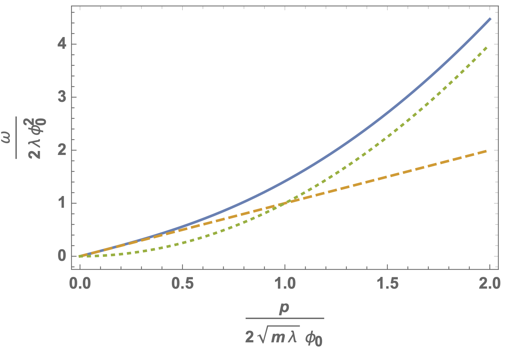
Bogoliulov excitations. It is also interesting to study small perturbations around the homogeneous field value \(\phi _0\). Let us write \begin{equation*} \varphi (x) = \phi _0 + \frac{1}{\sqrt{2}}\left [\phi _1(x) + i\,\phi _2 (x) \right ], \end{equation*} with real fields \(\phi _1(x)\) and \(\phi _2(x)\). The action in eq. \eqref{eq:microscopicactionBoseGasPotential} becomes (up to total derivatives) \begin{equation*} S= \int dt\;d^3x \left \{\phi _2 \partial _t \phi _1 + \frac{1}{2}\sum _{j=1}^2 \phi _j \frac{\vec{\nabla }^2}{2m}\phi _j -V\left (\phi ^2_0 + \sqrt{2}\phi _0\phi _1+ \tfrac{1}{2}\phi ^2_1 + \tfrac{1}{2}\phi ^2_2\right ) \right \}. \end{equation*} It is instructive to expand to quadratic order in the deviations from a homogeneous field \(\phi _1\) and \(\phi _2\). The quadratic part of the action reads \begin{equation*} S_2 = \int dt\;d^3x \left \{-\frac{1}{2}(\phi _1,\phi _2) \begin{pmatrix} -\frac{\vec{\nabla }^2}{2m}+2\lambda \phi ^2_0 & \partial _t \\ -\partial _t & -\frac{\vec \nabla ^2}{2m} \end{pmatrix} \begin{pmatrix} \phi _1 \\ \phi _2 \end{pmatrix} \right \}. \end{equation*} In momentum space, the matrix between the fields becomes \begin{equation*} G^{-1}(\omega ,\vec{p}) = \begin{pmatrix} \frac{\vec{p}^2}{2m}+ 2\lambda \phi ^2_0 & -i\omega \\ i\omega & \frac{\vec{p}^2}{2m} \end{pmatrix}. \end{equation*} In cases where the inverse propagator is a matrix, this holds also for the propagator. When the determinant of the inverse propagator has a zero-crossing, the propagator has a pole. This defines the dispersion relation for quasi-particle excitations, \begin{equation*} \det G^{-1}(\omega ,\vec{p})= 0. \end{equation*} Here this leads to \begin{equation*} -\omega ^2 + \left (\frac{\vec{p}^2}{2m} + 2\lambda \phi ^2_0\right )\frac{\vec{p}^2}{2m} = 0, \end{equation*} or \begin{equation} \omega = \sqrt{\left (\frac{\vec{p}^2}{2m}+2\lambda \phi ^2_0\right )\frac{\vec{p}^2}{2m}}. \label{eq:BogoliubovDispersionRelation} \end{equation} This is known as Bogoliubov dispersion relation.
Linear and quadratic regimes. For small momenta, such that \begin{equation*} \frac{\vec{p}^2}{2m} \ll 2\lambda \phi ^2_0, \end{equation*} one finds \begin{equation} \omega \approx \sqrt{\frac{\lambda \phi ^2_0}{m}}|\vec{p}|. \label{eq:BogoliubovDispersionRelationLowMomentum} \end{equation} In contrast, for \begin{equation*} \frac{\vec{p}^2}{2m} \gg 2\lambda \phi ^2_0, \end{equation*} one recovers the usual dispersion relation for non-relativistic particles \begin{equation} \omega \approx \frac{\vec{p}^2}{2m}. \label{eq:BogoliubovDispersionRelationLargeMomentum} \end{equation} The low-momentum region describes phonons (quasi-particles of sound excitations), while the large-momentum region describes normal particles.
Superfluidity. The fact that the dispersion relation is linear for small momenta is also responsible for another interesting phenomenon, namely superfluidity, a fluid motion without friction. To understand this consider an interacting Bose-Einstein condensate flowing past some body of through a capillary. If the energy and momentum of the fluid are \(E=E_0\) and \(\vec P=0\) in the fluid rest frame, they are \begin{equation*} E^\prime =E+ \vec P \vec v + \frac{1}{2}M \vec v^2 = E_0 + \frac{1}{2}M \vec v^2, \quad \quad \quad \vec P^\prime = \vec P + M \vec v = M \vec v, \end{equation*} in the rest frame of the body or capillary. We used here first the general transformation of energy \(E\) and momentum \(\vec P\) under Galilei boost transformations and then the particular values for the homogeneous fluid state.
Imagine now that we can create an excitation or quasi-particle in the fluid with energy \(\epsilon (\vec p)\) and momentum \(\vec p\). In the fluid rest frame we have now \(E=E_0+\epsilon (\vec p)\) and \(\vec P=\vec p\). The energy and momentum in the rest frame of the capillary are then \begin{equation*} E^\prime = E_0 + \epsilon (\vec p) + \vec p \cdot \vec v + \frac{1}{2}M \vec v^2, \quad \quad \quad \vec P^\prime = \vec p + M \vec v. \end{equation*} Comparison to the corresponding relation for the homogeneous state shows that the energy and momentum associated to the excitation are in the rest frame of the capiliary \(\epsilon (\vec p)+ \vec p \cdot \vec v\) and \(\vec p\), respectively.
Landau’s criterion for superfluidity. Now the point is that at small temperature, excitations will only be created in the fluid in appreciable numbers when it is energetically favorable, i.e. for \begin{equation*} \epsilon (\vec p)+ \vec p \cdot \vec v < 0, \end{equation*} such that the energy of the fluid is lowered. If this relation is not fulfilled for any momentum \(\vec p\), no excitations that could transport momentum out of a local fluid cell will be created. This means that there is no viscosity and the flow is superfluid. It follows that for friction to become possible, the fluid needs to have a fluid velocity larger than \begin{equation*} v_c = \underset{\vec p}{\text{min}} \frac{\epsilon (\vec p)}{|\vec p|}, \end{equation*} known as critical velocity. For the Bogoliubov dispersion relation \eqref{eq:BogoliubovDispersionRelation} the critical velocity equals the velocity of sound.
Summary. We have seen that relativistic quantum field theories can have a non-relativistic limit where Lorentz symmetry is replaced by Galilei symmetry. In the few-body limit this leads to the same predictions as quantum mechanics but the field theoretic formalism can have advantages, for example in the context of condensed matter theory. As an example we have discussed Bose-Einstein condensates where the low energy excitations are collective excitations of many particles in the form of sound waves or phonons. We have discussed here in particular the non-relativistic limit of a complex relativistic scalar field and have dropped the anti-particle excitations. One can also consider real relativistic scalar field theories which have a non-relativistic limit in terms of a complex scalar field, see for example [arXiv:2005.11359].