
Quantum field theory 1, lecture 13
7.3 Perturbation theory for interacting scalar fields
Partition function. Let us now consider a non-relativistic theory with the action \begin{equation*} S[\varphi ] = \int dt d^3 x \left \{\varphi ^*\left (i\partial _t + \frac{\nabla ^2}{2m} -V_0\right )\varphi -\frac{\lambda }{2}(\varphi ^*\varphi )^2\right \}. \end{equation*} We have rescaled the interaction parameter, \(\tfrac{\lambda }{4m^2} \to \lambda \). We introduce now the partition function in the presence of source terms \(J\) as \begin{equation*} Z[J] = \int D\varphi \; \exp \left [iS[\varphi ]+ i \int _x \left \{J^*(x)\varphi (x) + J(x)\varphi ^*(x)\right \}\right ], \end{equation*} with \(x = (t,\vec{x})\) and \(\int _x = \int dt \int d^3 x.\)
Source term. The source term can also be written in momentum space, \begin{equation*} \int _x \left \{J^*(x)\varphi (x) + J(x)\varphi ^*(x)\right \} = \int _p \left \{J^*(p)\varphi (p) + J(p)\varphi ^*(p)\right \}, \end{equation*} where \begin{equation*} \varphi (x) = \int _p e^{ipx} \varphi (p),\quad \quad \quad \varphi ^*(x) = \int _p e^{-ipx} \varphi ^*(p), \end{equation*} with \begin{equation*} \int _p = \int \frac{dp^0}{2\pi }\frac{d^3\vec{p}}{(2\pi )^3}, \end{equation*} and similar for the source \(J\). Because the source term has the same form in position and momentum space, we will sometimes simple write it as \begin{equation*} \int \left \{ J^* \varphi + \varphi ^* J \right \}. \end{equation*}
Correlation functions from functional derivatives. One can generate correlation functions from functional derivatives of \(Z[J]\), for example \begin{equation*} \begin{split} \langle \varphi (x) \varphi ^*(y) \rangle &= \langle 0| T\left \{\varphi (x)\varphi ^*(y)\right \}|0\rangle \\ &= \frac{\int D \varphi \;\varphi (x)\;\varphi ^*(y)\; e^{iS[\varphi ]}}{\int D\varphi \; e^{i S[\varphi ]}}\\ &= \left (\frac{(-i)^2}{Z[J]}\frac{\delta ^2}{\delta J^*(x) \delta J(y)} Z[J] \right )_{J=0}. \end{split} \end{equation*}
Functional derivatives in momentum space. One can also take functional derivatives directly in momentum space, for example \begin{equation*} \frac{\delta }{\delta J^*(P)}\; \exp \left [i\int \left \{J^*\varphi + \varphi ^* J\right \} \right ] = \frac{i}{(2\pi )^4}\; \varphi (p)\ \exp \left [i\int \left \{J^*\varphi + \varphi ^* J\right \} \right ]. \end{equation*} In this sense one can write \begin{equation*} \langle \varphi (p)\;\varphi ^*(q) \rangle = \left (\frac{(-i)^2}{Z[J]}(2\pi )^8\frac{\delta ^2}{\delta J^*(p) \delta J(q)} Z[J]\right )_{J=0}. \end{equation*}
Perturbation theory for partition function. Let us write the partition function formally as \begin{equation*}\begin{split} Z[J] = & \int D \varphi \; \exp \left [-i\frac{\lambda }{2}\int _x\left (-i\frac{\delta }{\delta J(x)}\right )^2 \left (-i\frac{\delta }{\delta J^*(x)}\right )^2\right ]\\ & \times \exp \left [iS_2[\varphi ]+ i\int \left \{J^*\varphi + \varphi ^*J\right \}\right ], \end{split}\end{equation*} where the quadratic action is \begin{equation*} S_2[\varphi ] = \int _x \varphi ^* \left (i \partial _t + \frac{\vec{\nabla }^2}{2m}-V_0\right )\varphi . \end{equation*} Note that when acting on the source term in the exponent, every functional derivative \(-i\frac{\delta }{\delta J(x)}\) results in a field \(\varphi ^*(x)\) and so on. In this way, the quartic interaction term has been separated and written in terms of derivatives with respect to the source field.
Separate interaction term. We can now pull it out of the functional integral and write \begin{equation*} Z[J] = \exp \left [-i\frac{\lambda }{2}\int _x\left (-i\frac{\delta }{\delta J(x)}\right )^2 \left (-i\frac{\delta }{\delta J^*(x)}\right )^2\right ] Z_2[J], \end{equation*} with the partition function for the quadratic theory \begin{equation*} Z_2[J] = \int D\varphi \; e^{i S_2[\varphi ] + i\int \left \{J^*\varphi +\varphi ^*J\right \}}. \end{equation*} The latter is rather easy to evaluate this in momentum space.
Quadratic part. One can write \begin{equation*} \begin{split} S_2 + \int \{J^*\varphi + \varphi ^*J\} &=\int _p \left \{-\varphi ^*\left (-p^0 + \tfrac{\vec{p}^2}{2m}+V_0\right )\varphi +J^*\varphi + \varphi ^* J\right \}\\ &=\int _p\left \{-\left [\varphi ^*-J^*\left (-p^0 + \tfrac{\vec{p}^2}{2m}+V_0\right )^{-1}\right ]\left (-p^0 + \tfrac{\vec{p}^2}{2m}+V_0\right ) \right .\\ & \left . \quad \quad \quad \times \left [\varphi -\left (-p^0 + \tfrac{\vec{p}^2}{2m}+V_0\right )^{-1} J\right ]\right \} \\ & \quad + \int _p \left \{J^*(p)\left (-p^0 + \tfrac{\vec{p}^2}{2m}+V_0\right )^{-1} J(p)\right \}. \end{split} \end{equation*} Note that the last term is independent of the field \(\varphi \) and can be pulled out of the functional integral.
Evaluate Gaussian integral. The functional integral over \(\varphi \) is of Gaussian form. One can shift the integration variable \begin{equation*} \left [\varphi -\left (-p^0 + \tfrac{\vec{p}^2}{2m}+V_0\right )^{-1} J\right ] \to \varphi , \end{equation*} and perform the functional integration in \(Z_2[\varphi ]\). It yields then only an irrelevant constant and as a result one finds \begin{equation*} Z_2[J] = \exp \left [i\int _p J^*(p)\left (-p^0 + \tfrac{\vec{p}^2}{2m}+V_0\right )^{-1} J(p)\right ]. \end{equation*}
Relating functional derivatives in position and momentum space. In the following it will be useful to write also the interaction term in momentum space. One may use \begin{equation*} \begin{split} & \frac{\delta }{\delta J(x)}= \int d^4 p \frac{\delta J(p)}{\delta J(x)}\frac{\delta }{\delta J(p)} = \int \frac{d^4 p}{(2\pi )^4} e^{-ipx} (2\pi )^4 \frac{\delta }{\delta J(p)} \\ & = \int \frac{d^4 p}{(2\pi )^4} e^{-ipx} \delta _{J(p)} = \int _p e^{-ipx}\delta _{J(p)}. \end{split} \end{equation*} Here we defined the abbreviation \begin{equation*} \delta _{J(p)} = (2\pi )^4 \frac{\delta }{\delta J(p)}. \end{equation*} In a similar way \begin{equation*} \frac{\delta }{\delta J^*(x)} = \int _p e^{ipx} \delta _{J^*(p)}. \end{equation*} We used also \begin{equation*} \int _x e^{ipx} = (2\pi )^4 \delta ^{(4)} (p). \end{equation*}
Perturbation series. One finds for the partition function \begin{equation} \begin{split} Z[J] &= \exp \left [-i \frac{\lambda }{2} \int _x \left (\tfrac{\delta }{\delta J(x)}\right )^2 \left (\tfrac{\delta }{\delta J^* (x)}\right )^2\right ] Z_2[J]\\ &= \exp \left [-i \frac{\lambda }{2}\int _{k_1...k_4}\left \{(2\pi )^4 \delta ^4(k_1+k_2-k_3-k_4) \delta _{J(k_1)}\delta _{J(k_2)}\delta _{J^*(k_3)}\delta _{J^*(k_4)}\right \}\right ] \\ & \quad \times \exp \left [i\int _p J^*(p)\left (-p^0 + \tfrac{\vec{p}^2}{2m}+V_0\right )^{-1} J(p)\right ]. \end{split} \label{eq:partitionFunctionPerturbativeSeries} \end{equation} One can now expand the exponential to obtain a formal perturbation series in \(\lambda \).
S-matrix element. Let us now come back to the S-matrix element for \(2\to 2\) scattering \begin{equation*} \begin{split} & \langle \vec{q}_1,\vec{q}_2; \text{out}| \vec{p}_1,\vec{p}_2;\text{in}\rangle \\ & =i^4 \left [-q^0_1+\tfrac{\vec{q}^2_1}{2m}+V_0\right ]\left [-q^0_2+\tfrac{\vec{q}^2_2}{2m}+V_0\right ]\left [-p^0_1+\tfrac{\vec{p}^2_1}{2m}+V_0\right ]\left [-p^0_2+\tfrac{\vec{p}^2_2}{2m}+V_0\right ] \\ & \quad \quad \times \left \langle \varphi (q_1)\varphi (q_2)\varphi ^*(p_1)\varphi ^*(p_2) \right \rangle \\ & =i^4 \left [-q^0_1+\tfrac{\vec{q}^2_1}{2m}+V_0\right ]\left [-q^0_2+\tfrac{\vec{q}^2_2}{2m}+V_0\right ]\left [-p^0_1+\tfrac{\vec{p}^2_1}{2m}+V_0\right ]\left [-p^0_2+\tfrac{\vec{p}^2_2}{2m}+V_0\right ] \\ & \quad \quad \times \left (\frac{1}{Z[J]} \delta _{J^*(q_1)}\delta _{J^*(q_2)}\delta _{J(p_1)}\delta _{J(p_2)} Z[J]\right )_{J=0}. \end{split} \end{equation*} If we now insert the perturbation expansion for Z[J], we can concentrate on the contribution at order \(\lambda ^1=\lambda \), because at order \(\lambda ^0 = 1\) we have only the trivial S-matrix element for no scattering that we already discussed.
Order \(\lambda \). At order \(\lambda \) we have different derivatives acting on \(Z_2 [J]\),
- \(\delta _{J(p_1)}\)for incoming particles with momentum \(\vec{p}_1\)
- \(\delta _{J^*(q_1)}\)for outgoing particle with momentum \(\vec{q}_1\)
- \(\delta _{J(k)}\)and \(\delta _{J^*(k)}\) for the interaction term.
Propagator. At the end, all these derivatives are evaluated at \(J=J^*=0\). Therefore, there must always be derivatives \(\delta _J\) and \(\delta _J^*\) acting together on one integral appearing in \(Z_2[J]\). Note that \begin{equation*}\begin{split} & \delta _{J(p_1)}\delta _{J^*(q_1)}\left [i\int _p J^*(p)\left (-p^0 + \tfrac{\vec{p}^2}{2m}+V_0\right )^{-1} J(p)\right ] \\ & =i\left (-p_1^0 + \tfrac{\vec{p}^2_1}{2m}+V_0\right )^{-1} (2\pi )^4 \delta ^{(4)}(p_1-q_1). \end{split} \end{equation*}
Momentum conservation. If two derivatives representing external particles would hit the same integral in \(Z_2[J]\), one would have no scattering because \(\vec{p}_1 =\vec{q}_1\) and as a result of momentum conservation then also \(\vec{p}_2 =\vec{q}_2\). This is no real scattering. Only if a derivative representing an incoming or outgoing particle is combined with a derivative from the interaction term, this is avoided.
Resulting contribution to S-matrix. By doing the algebra one finds at order \(\lambda \) the term for scattering \begin{equation*} \langle \vec{q}_1,\vec{q}_2; \text{out}| \vec{p}_1,\vec{p}_2;\text{in}\rangle = -i \frac{\lambda }{2}4 \, (2\pi )^4 \delta ^{(4)} (q_1 +q_2 -p_1 -p_2). \end{equation*} The factor \(4=2\times 2\) comes from different ways to combine functional derivatives with sources.
Momentum conservation. The overall Dirac function makes sure that the incoming four-momentum equals the out-going four-momentum, \begin{equation*} p^{\text{in}}= p_1 + p_2 = q_1+q_2= p^{\text{out}}. \end{equation*}
Transition amplitude. Quite generally, one can define for the non-trivial part of an S-matrix \begin{equation*} \langle \beta ;\text{out}|\alpha ;\text{in}\rangle = (2\pi )^4 \delta ^{(4)} (p^{\text{out}}-p^{\text{in}}) \, i \,{\cal T}_{\beta \alpha }. \end{equation*} Together with the trivial part from “no scattering”, one can write \begin{equation*} S_{\beta \alpha } = \delta _{\beta \alpha } + (2\pi )^4 \delta ^{(4)} (p^{\text{out}}-p^{\text{in}}) \, i \,{\cal T}_{\beta \alpha }. \end{equation*} By comparison of expressions we find for the \(2\to 2\) scattering of non-relativistic bosons at lowest order in \(\lambda \) simply \begin{equation*}{\cal T} = -2\lambda , \end{equation*} independant of momenta. More generally, the transition amplitude \(\cal T\) is expected to depend on the momenta of incoming and outgoing particles.
Diagrammatic representation. To keep the overview over a calculation it is sometimes useful to introduce a graphical representation. For the perturbation series discussed above we may represent incoming particles by
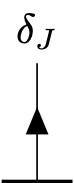 \( = i\left [-p^0_1 + \frac{\vec{p}^2_1}{2m} + V_0\right ] \delta _{J(p_1)} = i\left [-p^0_1 + \frac{\vec{p}^2_1}{2m} + V_0\right ] \frac{\delta }{\delta{J(p_1)}},\)
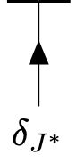 \(= i\left [-q^0_1 + \frac{\vec{q}^2_1}{2m} + V_0\right ] \delta _{J^*(q_1)} = i\left [-q^0_1 + \frac{\vec{q}^2_1}{2m} + V_0\right ] \frac{\delta }{\delta{J^*(q_1)} }.\)
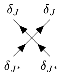 \(= -i \frac{\lambda }{2}\int _{k_1...k_4}\left \{(2\pi )^4 \delta ^4(k_1+k_2-k_3-k_4) \delta _{J(k_1)}\delta _{J(k_2)}\delta _{J^*(k_3)}\delta _{J^*(k_4)}\right \},\)
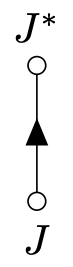 \(= i\int _p J^*(p)\left (-p^0 + \frac{\vec{p}^2}{2m}+V_0\right )^{-1} J(p).\)