Quantum field theory 1, lecture 16
8.3 Yukawa theory
Yukawa theory. Let us now investigate a theory for a non-relativistic fermion with spin \(1/2\) and a real, relativistic scalar boson \begin{equation*} S = \int dt d^3x \left \{-\bar{\psi }\left (-i\partial _t - \tfrac{\vec{\nabla }^2}{2m} +V_0 - i\epsilon \right ) \psi -\tfrac{1}{2} \phi \left (\partial ^2_{t} - \vec{\nabla }^2 +M^2 -i\epsilon \right )\phi -g\phi \bar{\psi }\psi \right \}. \end{equation*}
Partition function for Yukawa theory. We will discuss this theory in terms of the partition function \begin{equation*} Z[\bar{\eta },\eta , J] = \int D\bar{\psi }D\psi D\phi \; e^{i S[\bar{\psi },\psi ,\phi ] + i\int _x\{\bar{\eta }\psi + \bar{\psi }\eta +J\phi \} } . \end{equation*} As usual, by taking functional derivatives with respect to the source fields, one can obtain various correlation functions. Our strategy will be to perform a perturbation expansion in the cubic term \(\sim g\).
Quadratic action. Let us first concentrate on the quadratic theory and the corresponding partition function derived from the action \begin{equation*} S_2 = \int dt d^3 x \left \{-\bar{\psi }\left (-i\partial _t -\frac{\vec{\nabla }^2}{2m}+V_0-i\epsilon \right )\psi -\frac{1}{2}\phi (\partial ^2_{t} - \vec{\nabla }^2+M^2 -i\epsilon )\phi \right \} . \end{equation*} By doing the Gaussian integration one finds \begin{equation*} \begin{split} Z_2 [\bar{\eta },\eta , J] &= \int D\bar{\psi }D\psi D\phi \; \exp \left [iS_2 + i\int _x \left \{\bar{\eta }\psi +\bar{\psi }\eta +J\phi \right \}\right ]\\ &= \exp \left [i\int d^4x d^4y \left \{\bar{\eta }(x) \Upsilon (x-y)\eta (y) +\frac{1}{2} J(x) \Delta (x-y) J(y)\right \} \right ] \end{split} \end{equation*} where \(\Upsilon (x-y)\) is the Greens function for fermions. For the scalar bosons, the Green function is \begin{equation*} \Delta (x-y) = \int \frac{d^4p}{(2\pi )^4}\frac{1}{-(p^0)^2 + \vec{p}^2 +M^2 - i\epsilon } e^{ip(x-y)}. \end{equation*}
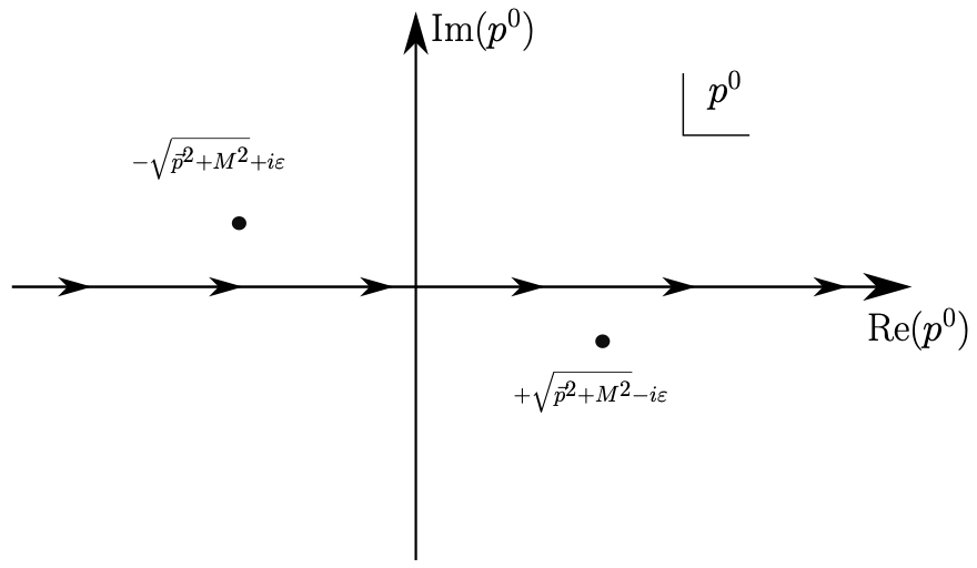
Time-ordered boundary conditions or \(i\epsilon \) prescription. Again, the \(i\epsilon \) term makes sure that the Greens function corresponds to the time-ordered or Feynman boundary conditions. One can also obtain this from a careful consideration of analytic continuation from Euclidean space to real time or Minkowski space. Note that the \(i\epsilon \) term has in the functional integral the form \begin{equation*} e^{iS} = e^{i [\ldots + i\epsilon \int _x \phi ^2 (x)]} = e^{-\epsilon \int _x \phi (x)^2 + i\ldots }. \end{equation*} This is the same suppression term that also appears in the Euclidean functional integral. It makes sure that functional integrals are converging and that the theory approaches the ground state on long time scales.
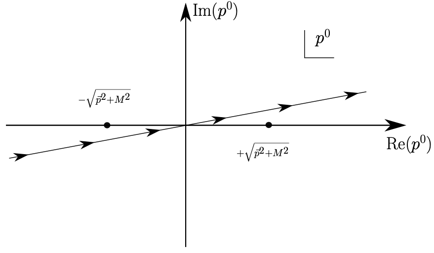
In the complex plane, positions of poles are shifted slightly away from the real axis. This is illustrated in the left panel of figure 1. In fact this is equivalent to keeping the poles at \(p^0 = \pm \sqrt{\vec{p}^2+M^2}\) but moving slightly in the integration contour. This is illustrated in the right panel of figure 1.
Time ordered or Feynman propagator in position space. Let us use either of these prescriptions to calculate the scalar field propagator in position space \begin{equation*} \Delta (x-y) = \int \frac{dp^0}{2\pi } \frac{d^3p}{(2\pi )^3} \frac{e^{-i p^0(x^0-y^0)+i\vec{p}(\vec{x}-\vec{y})}}{ \left (-p^0 + \sqrt{\vec{p}^2 +M^2} -i\epsilon \right ) \left (p^0 + \sqrt{\vec{p}^2 + M^2} -i\epsilon \right )}. \end{equation*} The strategy will be to close the integration contour at \(|p^0| \to \infty \) and to use the residue theorem. First, for \(x^0-y^0 > 0\), we can close the contour in the lower half of the complex \(p^0\)-plane because \(e^{-ip^0(x^0-y^0)} \to 0\) there. There is then only the residue at \(p^0 = \sqrt{\vec{p}^2+M^2}\) inside the integration contour (the \(i\epsilon \) has already been dropped there). The residue theorem gives for the \(p^0\) integral (for \(x^0-y^0 > 0\)) \begin{equation*} \Delta (x-y) = \int \frac{d^3 p}{(2\pi )^3} \frac{i}{2\sqrt{\vec{p}^2+ M^2}} \; e^{-i \sqrt{\vec{p}^2 +M^2}(x^0-y^0)}\;e^{i\vec{p}(\vec{x} - \vec{y})}. \end{equation*} In contrast, for \(x^0 -y^0 < 0\) we need to close the \(p^0\)-integral in the upper half of the complex \(p^0\) plane. The residue theorem given then (for \( \text{for}\;\; x^0-y^0 < 0\))\begin{equation*} \Delta (x-y) = \int \frac{d^3 p}{(2\pi )^3} \frac{i}{2\sqrt{\vec{p}^2+ M^2}} \; e^{i \sqrt{\vec{p}^2 +M^2}(x^0-y^0)}\;e^{i\vec{p}(\vec{x} - \vec{y})}. \end{equation*} These results can be combined to \begin{equation*} \begin{split} \Delta (x-y) = & \int \frac{d^3 p}{(2\pi )^3} \frac{i}{2\sqrt{\vec{p}^2+ M^2}} e^{-i \sqrt{\vec{p}^2 +M^2} | x^0-y^0 |+i\vec{p}(\vec{x} - \vec{y})}\\ = & i\theta (x^0 - y^0) \int \frac{d^3 p}{(2\pi )^3} \frac{1}{2\sqrt{\vec{p}^2+ M^2}} e^{-i \sqrt{\vec{p}^2 +M^2}(x^0-y^0)+i\vec{p}(\vec{x} - \vec{y})}\\ &+ i\theta (y^0-x^0) \int \frac{d^3 p}{(2\pi )^3} \frac{1}{2\sqrt{\vec{p}^2+ M^2}} e^{i \sqrt{\vec{p}^2 +M^2}(x^0-y^0)+i\vec{p}(\vec{x} - \vec{y})}. \end{split} \end{equation*} One can understand the first term as being due to particle-type excitations, while the second is due to anti-particle-type excitations. The above Greens function is known as time ordered or Feynmann propagator.
Propagator for non-relativistic fermions. For the non-relativistic fermion, the propagator integral over \(p^0\) has just a single pole at \(p^0 = \frac{\vec{p}^2}{2m}+ V_0 - i\epsilon ,\) \begin{equation*} \Upsilon (x-y) = \mathbb{1} \int \frac{dp^0}{2\pi }\frac{d^3 p}{(2\pi )^3} \frac{1}{-p^0 +\frac{\vec{p}^2}{2m}+V_0 - i\epsilon }e^{-ip^0(x^0-y^0)+ i\vec{p}(\vec{x} - \vec{y}).} \end{equation*} When \(x^0-y^0 > 0\) the contour can be closed below the real \(p^0\)-axis, leading to \begin{equation*} \Upsilon (x-y) = i\; \mathbb{1} \int \frac{d^3p}{(2\pi )^3}\; e^{-i{\big (} \frac{\vec{p}^2}{2m}+V_0{\big )}(x^0-y^0) + i\vec{p}(\vec{x} - \vec{y})} \quad \quad \quad (x^0 - y^0 > 0). \end{equation*} In contrast, for \(x^0 - y^0 < 0,\) the contour can be closed above and there is no contribution at all. In summary \begin{equation*} \Upsilon (x-y) = i\;\theta (x^0-y^0)\; \mathbb{1} \int \frac{d^3p}{(2\pi )^3}\; e^{-i{\big (} \frac{\vec{p}^2}{2m}+V_0{\big )}(x^0-y^0) + i\vec{p}(\vec{x} - \vec{y})}. \end{equation*} As a consequence of the absence of anti-particle-type excitations, the time-ordered and retarded propagators agree here.
Propagator and correlation functions. Let us also note the relation between propagators and correlation functions. For the free (quadratic) theory one has in the fermionic sector \begin{equation*} \begin{split} \left \langle \psi _a (x) \bar{\psi }_b (y)\right \rangle &= \left (\frac{1}{Z_2} \frac{\delta }{\delta \bar{\eta }_a (x)}\frac{\delta }{\delta \eta _b (y)} Z_2[\bar{\eta }, \eta , J]\right )_{\bar{\eta } = \eta = J = 0}\\ &= -i \Upsilon _{ab} (x-y), \end{split} \end{equation*} Note that some care is needed with interchanges of Grassmann variables to obtain this expression. Similarly for the bosonic scalar field \begin{equation*} \begin{split} \left \langle \phi (x) \phi (y) \right \rangle &= \left (\frac{1}{Z_2} \frac{\delta }{\delta J(x)}\frac{\delta }{\delta J(y)} Z_2[\bar{\eta }, \eta , J]\right )_{\bar{\eta } = \eta = J = 0}\\ &= -i \Delta (x-y). \end{split} \end{equation*}
Wick’s theorem. More generally one finds for the free theory \begin{equation*} \begin{split} \left \langle \phi (x_1) \ldots \phi (x_n) \right \rangle &= \left ( \frac{1}{Z_2} \left (-i \frac{\delta }{\delta J(x_1)}\right )\cdots \left (-i\frac{\delta }{\delta J(x_n)}\right )Z_2[\bar \eta , \eta , J]\right )_{\bar{\eta }= \eta = J =0}\\ &= \sum _{\text{pairings}}\left [-i \Delta (x_{j_1} - x_{j_2})\right ] \cdots \left [-i \Delta (x_{j_{n-1}}-x_{j_n})\right ]. \end{split} \end{equation*} The sum in the last line goes over all possible ways to distribute \(x_1, \ldots , x_n\) into pairs \((x_{j_1}, x_{j_2})\), \((x_{j_3}, x_{j_4})\), \(\ldots \), \((x_{j_{n-1}}, x_{j_n})\). This result is known as Wick’s theorem. It follows directly from the combinatorics of functional derivatives acting on \(Z_2\).
For example, \begin{equation*} \begin{split} \left \langle \phi (x_1)\; \phi (x_2)\; \phi (x_3) \phi (x_4) \right \rangle = & [-i \Delta (x_1 - x_2)][-i \Delta (x_3 - x_4)]\\ & + [-i \Delta (x_1 - x_3)][-i \Delta (x_2 - x_4)]\\ &+ [-i\Delta (x_1 - x_4)] [-i \Delta (x_2 - x_3)]. \end{split} \end{equation*}
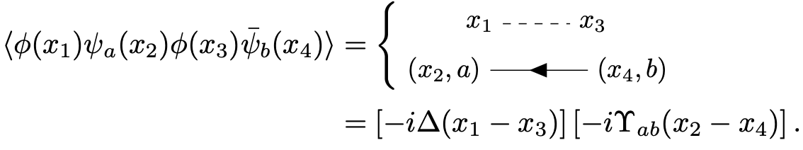
In a similar way correlation functions involving \(\bar{\psi }\) and \(\psi \) can be written as sums over the possible ways to pair \(\psi \) and \(\bar{\psi }\). For example \begin{equation*} \begin{split} \left \langle \psi _{a_1}(x_1) \psi _{a_2}(x_2) \bar{\psi }_{a_3}(x_3) \bar{\psi }_{a_4}(x_4) \right \rangle = & -\left \langle \psi _{a_1}(x_1) \bar{\psi }_{a_3}(x_3)\right \rangle \left \langle \psi _{a_2}(x_2) \bar{\psi }_{a_4}(x_4) \right \rangle \\ &+\left \langle \psi _{a_1}(x_1) \bar{\psi }_{a_4}(x_4)\right \rangle \left \langle \psi _{a_2}(x_2) \bar{\psi }_{a_3}(x_3) \right \rangle \\ = & -[-i \Upsilon _{a_1a_3}(x_1-x_3)][-i\Upsilon _{a_2a_4}(x_2-x_4)]\\ &+[-i \Upsilon _{a_1a_4}(x_1-x_4)][-i \Upsilon _{a_2a_3}(x_2-x_3)]. \end{split} \end{equation*} Note that correlation functions at quadratic level (for the free theory) need to involve as many fields \(\psi \) as \(\bar{\psi }\), otherwise they vanish. Similarly, \(\phi \) must appear an even number of times. For mixed correlation functions one can easily separate \(\phi \) from \(\psi \) and \(\bar{\psi }\) at quadratic level, because \(Z_2[\bar \eta , \eta , J]\) factorizes. For example, \begin{equation} \left \langle \phi (x_1)\;\psi _a(x_2)\;\phi (x_3) \bar{\psi }_b(x_4) \right \rangle = [-i\Delta (x_1 - x_3)][-i\Upsilon _{ab}(x_2 - x_4)]. \label{eq:fermion2boson2correlation} \end{equation}
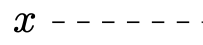
Graphical representation. It is useful to introduce also a graphical representation. We will represent the scalar propagator by a dashed line
\(-i\Delta (x-y) = \)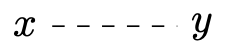
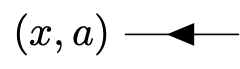
\(-i\Upsilon _{ab}(x-y)= \)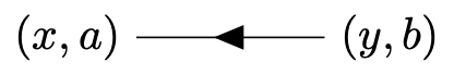
Perturbation theory in \(g\).
Let us now also consider the interaction terms in the action. In the functional integral it contributes
according to \begin{equation*} e^{iS[\bar{\psi },\psi ,\phi ]}= e^{iS_2[\bar{\psi },\psi ,\phi ]} \; \exp \left [-i g \int d^4x \phi (x) \bar{\psi }_a (x) \psi _a (x)\right ]. \end{equation*}
We can assume that \(g\) is small and simply expand the exponential where it appears. This will add field
factors \(\sim \phi (x) \bar{\psi }_a (x) \psi _a(x)\) to correlation functions with an integral over \(x\) and an implicit sum over the spinor index \(a\). The
resulting expression involving correlation functions can then be evaluated as in the free theory. For
example, \begin{equation*} \begin{split} \left \langle \phi (x_1) \psi _b(x_2) \bar{\psi }_c(x_3) \right \rangle &= \left \langle \phi (x_1) \psi _b(x_2) \bar{\psi }_c(x_3) \right \rangle _0\\ &\qquad +\left \langle \phi (x_1) \psi _b(x_2) \bar{\psi }_c(x_3) \left [-ig\int _y \phi (y) \bar{\psi }_a(y) \psi _a(y)\right ]\right \rangle _0 + \ldots \end{split} \end{equation*}
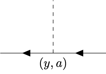
The index \(0\) indicates that the correlation functions get evaluated in the free theory. Graphically, we can
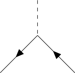
represent the interaction term as a vertex
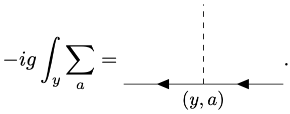 For each such vertex we need to include a factor \(-ig\) as well as an integral over the space-time variable \(y\) and
the spinor index \(a\).
For each such vertex we need to include a factor \(-ig\) as well as an integral over the space-time variable \(y\) and
the spinor index \(a\).
Three point function.
To order \(g\), we find for the example above
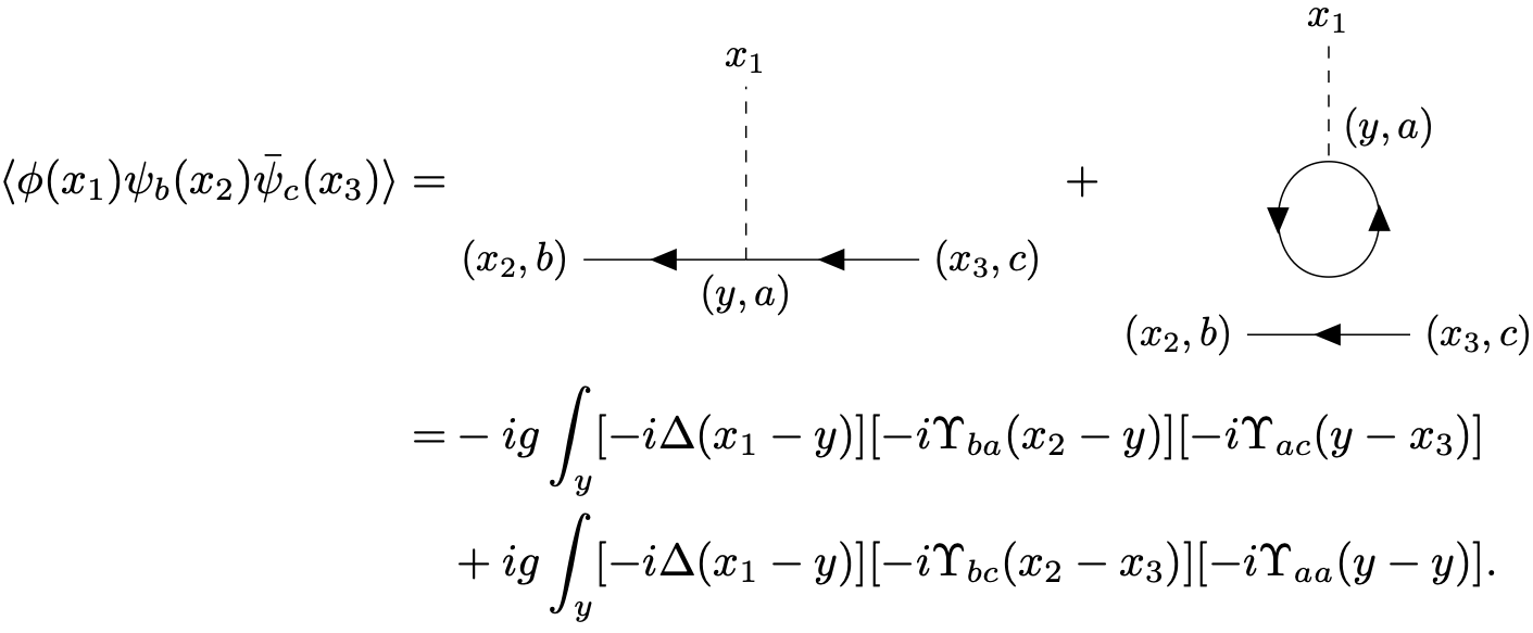 The sign in the last line is due to an interchange of Grassmann fields. The last expression involves the
fermion propagator for vanishing argument \begin{equation*} \Upsilon _{ab}(0) = \delta _{ab} \int \frac{d^4 p}{(2\pi )^4}\frac{1}{-p^0 +\tfrac{\vec{p}^2}{2m}+V_0-i\epsilon } = i\theta (0)\delta _{ab} \delta ^{(3)}(0). \end{equation*}
We will set here \(\theta (0) = 0\) so that the corresponding contribution vanishes. In other words, we will interpret
\begin{equation*} \Upsilon _{ab}(0) = \lim _{\Delta t\to 0} \Upsilon _{ab}(-\Delta t, \vec 0 ) = 0. \end{equation*}
Although this is a little ambiguous at this point, it turns out that this is the right way to
proceed.
The sign in the last line is due to an interchange of Grassmann fields. The last expression involves the
fermion propagator for vanishing argument \begin{equation*} \Upsilon _{ab}(0) = \delta _{ab} \int \frac{d^4 p}{(2\pi )^4}\frac{1}{-p^0 +\tfrac{\vec{p}^2}{2m}+V_0-i\epsilon } = i\theta (0)\delta _{ab} \delta ^{(3)}(0). \end{equation*}
We will set here \(\theta (0) = 0\) so that the corresponding contribution vanishes. In other words, we will interpret
\begin{equation*} \Upsilon _{ab}(0) = \lim _{\Delta t\to 0} \Upsilon _{ab}(-\Delta t, \vec 0 ) = 0. \end{equation*}
Although this is a little ambiguous at this point, it turns out that this is the right way to
proceed.
Feynmann rules in position space. To calculate a field correlation function in position space we need to
- have a scalar line ending on \(x\) for a factor \(\phi (x)\),
- have a fermion line ending on \(x\) for a factor \(\psi _a(x)\),
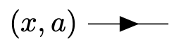
- have a fermion line starting on \(x\) for a factor
- include a vertex \(-ig\int _y\) for every order \(g\),
 with integral over \(y\).
- connect lines with propagators \([-i\Delta (x-y)]\) or \([-i\Upsilon _{ab}(x-y)]\)
- determine the overall sign for interchanges of fermionic fields.
S-matrix elements from amputated correlation functions. To calculate S-matrix elements from correlation functions, we need to use the LSZ formula. For an outgoing fermion, we need to apply the operator \begin{equation*} i\left [-i\partial _t -\tfrac{\vec{\nabla }^2}{2m}+V_0\right ]\left \langle \cdots \psi _a(x)\cdots \right \rangle \end{equation*} and also go to momentum space by a Fourier transform \begin{equation*} \int _x e^{+i\omega _p x^0-i\vec{p}\vec{x}}. \end{equation*} The operator simply removes the propagator leading to \(x\), because of \begin{equation*} \begin{split} & i\left [-i\partial _{x^0} - \tfrac{\vec{\nabla }^2_x}{2m}+V_0\right ]\; \left [-i\Upsilon _{ab}(x-y)\right ] \\ &=\delta _{ab}\int \frac{d^4p}{(2\pi )^4} e^{ip(x-y)} \frac{-p^0+\tfrac{\vec{p}^2}{2m}+V_0}{-p^0+\tfrac{\vec{p}^2}{2m}+V_0} = \delta _{ab} \delta ^{(4)}(x-y). \end{split} \end{equation*} One says that the correlation function is “amputated” because the external propagator has been removed.
Feynman rules for S-matrix elements in momentum space. Moreover, all expressions are brought back to momentum space. One can formulate Feynmann rules directly for contributions to \(i{\cal T}\) as follows.
- Incoming fermions are represented by an incoming line
 (to be read from right to left)
associated with a momentum \(\vec{p}\) and energy \(\omega _{\vec{p}} = \tfrac{\vec{p}^2}{2m}+V_0\).
(to be read from right to left)
associated with a momentum \(\vec{p}\) and energy \(\omega _{\vec{p}} = \tfrac{\vec{p}^2}{2m}+V_0\).
- Outgoing fermions are represented by an outgoing line
- Incoming or outgoing bosons are represented by
 and
and  respectively.
- Vertices
 contribute a factor \(-ig\).
- Internal lines that connect two vertices are represented by Feynmann propagators in momentum
space, e. g.

- Energy and momentum conservation are imposed on each vertex.
- For tree diagrams, all momenta are fixed by energy and momenta conservation. For loop diagrams one must include an integral over the loop momentum \(l_j\) with measure \(\tfrac{d^4 l_j}{(2\pi )^4}.\)
- Some care is needed to fix overall signs for fermions.
- Some care is needed to fix overall combinatoric factors from possible interchanges of lines or functional derivatives.
For the last two points it is often useful to go back to the algebraic expressions or to have some experience. We will later discuss very useful techniques based on generating functionals.
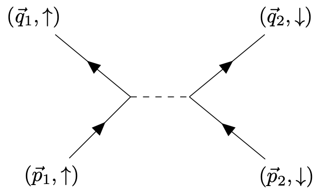
Fermion-fermion scattering.
We will now discuss an example, the scattering of (spin polarized) fermions of each other. The
tree-level diagram is
Limits of large and small mass. Note that for \(g^2 \to \infty ,\) \(M^2 \to \infty \) with \(g^2/M^2\) finite, \(\cal T\) becomes independent of momenta. This resembles closely the \(\lambda (\phi ^* \phi )^2\) interaction we discussed earlier for bosons. More, generally, one can write \begin{equation*} (\vec{p}_1 - \vec{q}_1)^2 = 2|\vec{p}_1|^2 (1-\cos (\vartheta )) = 4|\vec{p}_1|^2 \sin ^2(\vartheta /2), \end{equation*} where we used \(|\vec{p}_1| = |\vec{q}_1|\) in the center of mass frame and \(\vartheta \) is the angle between \(\vec{p}_1\) and \(\vec{q}_1\) (incoming and outgoing momentum of the spin \(\uparrow \) particle). For the differential cross-section \begin{equation*} \frac{d\sigma }{d \Omega _{q_1}} = \frac{|{\cal T}|^2 m^2}{16 (\pi )^2}, \end{equation*} we find \begin{equation*} \frac{d\sigma }{d\Omega _{q_1}} = \frac{g^4 m^2}{16 \pi ^2}\left [\frac{1}{4 \vec{p}_{1}^{2} \sin ^2(\vartheta /2) +M^2}\right ]^2 . \end{equation*} Another interesting limit is \(M^2 \to 0\). One has then \begin{equation*} \frac{d\sigma }{d\Omega _{q_1}} = \frac{g^4 m^2}{64 \pi ^2 |\vec{p}_1|^4}\frac{1}{\sin ^4(\vartheta /2)}. \end{equation*} This is the differential cross-section form found experimentally by Rutherford. It results from the exchange of a massless particle or force carrier which is here the scalar boson \(\phi \) and in the case of Rutherford experiment (scattering of \(\alpha \)-particles on Gold nuclei) it is the photon. This cross section has a strong peak at forward scattering \(\vartheta \to 0,\) and for \(\vec{p}^2 \to 0\). These are known as colinear and soft singularities. Note that they are regulated by a small, nonvanishing mass \(M > 0\).