
Quantum field theory 1, lecture 18
Lorentz algebra. The product of two group elements is again a group element. From this we can conclude that the commutator of two generators must again be a generator. In general we can therefore write \begin{equation} [T_x, T_y] = if_{xyz}T_z, \label{eq:commutatorGenerators} \end{equation} where the sum over \(z\) is implied. The quantities \(f_{xyz}\) are called the structure constants of a group. The structure constants are central elements for Lie groups. They encode the algebraic properties. For the example of the three-dimensional rotation group SO(3) with \(z=1..3\) one has \(f_{xyz}=\epsilon _{xyz}\). This tells us that the order matters for a sequence of rotations around different axes.
The central relation \eqref{eq:commutatorGenerators} can be shown as follows. Let us write two transformations \(\Lambda _1\) and \(\Lambda _2\) as \begin{equation*} \Lambda _1=e^{iA}, \quad \Lambda _2=e^{iB},\quad \quad \quad A= \epsilon ^{(A)}_z T_z,\quad B = \epsilon ^{(B)}_y T_y. \end{equation*} The combined transformation, \begin{equation*} \Lambda _1^{-1} \Lambda _2^{-1} \Lambda _1 \Lambda _2=e^{-iA} e^{-iB} e^{iA} e^{iB} = e^{iC}, \end{equation*} is again an element of the group and therefore \(C = \epsilon ^{(C)}_w T_w\). We use \begin{equation*} e^{iA}e^{iB} = e^{iB} e^{iA} + [B,A]+ \ldots \end{equation*} and expand the combined transformation in lowest non-trivial order \(\epsilon ^2\) \begin{equation} \begin{split} \mathbb{1}+[B,A] &= \mathbb{1} + iC, \quad [B,A] = iC,\\ -\epsilon ^{(B)}_y \epsilon ^{(A)}_z [T_y, T_z] &= i\tilde{\epsilon }^{(C)}_w T_w. \end{split} \label{eq:tildeepsilon} \end{equation} Here \(\tilde{\epsilon }^{(C)}_w\) are real parameters of the order \(\epsilon ^2\). The matrix equation \eqref{eq:tildeepsilon} can only be true if the commutators \(-i [T_z,T_y]\) are linear combinations of generators, \begin{equation*} -i[T_z, T_y] = c^{(zy)}_w T_w. \end{equation*} The coefficients \(c^{(zy)}_w = f_{zyw}\) can be identified with the structure constants.
Example.
As an example, we consider a rotation in three dimensional space. We want to rotate a
system
\(\bullet \) by an angle \(\alpha \) around the \(y\)-axis,
\(\bullet \) by an angle \(\beta \) around the \(x\)-axis,
\(\bullet \) by an angle \(-\alpha \) around the \(y\)- axis,
\(\bullet \) and finally by an angle \(-\beta \) around the \(x\)-axis.
The result of a product of infinitesimal rotations is again an infinitesimal rotation, \begin{equation*} \begin{split} &\left (1-i\beta T_x - \tfrac{1}{2}\beta ^2 T^2_x\right )\left (1-i\alpha T_y - \tfrac{1}{2}\alpha ^2 T^2_y\right )\left (1+i\beta T_x - \tfrac{1}{2}\beta ^2 T^2_x\right )\left (1+i\alpha T_y - \tfrac{1}{2}\alpha ^2 T^2_y\right ) \\ &= 1-\alpha \beta (T_x T_y - T_y T_x) =1-i\alpha \beta T_z \end{split} \end{equation*}
The first order is zero, and the terms \(\propto T^2_x\) and \(\propto T^2_y\) cancel, too. The product \(\alpha \beta \) is the parameter of the resulting
infinitesimal transformation.
For the special case of a rotation in three dimensional space the commutation relation \begin{equation*} [T_1, T_2]= iT_3 \end{equation*} follows directly from the multiplication of the matrices specified before. More generally, the generators of rotations obey \begin{equation*} [T_k, T_l]= i\epsilon _{klm} T_m \quad \text{for}\quad k,l,m \in \{1,2,3\}. \end{equation*}
The calculation of this example gives us already some commutation relations of the generators of the Lorentz group, if we consider the \(T_i\) as 4 x 4 matrices with zeroes in all elements of the first column and row. This is of course not surprising, as the three dimensional rotations are a subgroup of the Lorentz group. The other structure constants \(f_{xyz}\) where one element of \(x,y,z\) is \(0\) can also be found from the specified matrices. We will indicate them later explicitly.
9.4 Representations of the Lorentz group
The spin matrices \(s_k=\tfrac{1}{2}\tau _k\) are given by the Pauli matrices \(\tau _k\). The commutation relations for the Pauli matrices imply that the spin matrices obey precisely the same commutation relations as the generators of the rotation group \(SO(3)\), \begin{equation*} \begin{split} [\tau _k, \tau _l] &= 2i\epsilon _{klm} \tau _m,\quad [s_k, s_l] = i\epsilon _{klm} s_m. \end{split} \end{equation*}
We can define \(3\times 3\)-matrices \(\tilde{T}_k\) by omitting in the matrices defined before the first row and column. The \(3\times 3\)-matrices \(\tilde{T}_k\) and the spin matrices \(s_k\) obey the same commutation relation. They correspond to different representations of the rotation group. The matrices \(\tilde{T}_m\) are a three-dimensional and the matrices \(\tau _m/2\) are a two-dimensional representation of the group \(SO(3)\). Different representations of a group correspond to different sets of matrices that obey the same product rules for their multiplication, as given by the product rule for the abstract group elements. The dimension of the different matrix-representations can differ. For continuous transformations the transformation rules of a Lie group are encoded in the commutator relations for the generators. Two different sets of generators with the same commutation relations generate two different representations of the group.
d-dimensional representation. For a \(d\)-dimensional representation the set of \(d \times d\)- matrices \(T_z\) obeys the commutation relations of a given group. In the physics literature, one often uses the representation to design (somewhat improperly) also a \(d\)-component object on which the matrices \(T_z\) act.
Representations of the Lorentz group. Let us summarize what we know about the Lorentz group: It is \(SO(1,3)\) and is generated by a set of 6 independent matrices \(T_z\), which obey the commutation relations \begin{equation*} [T_x,T_y] = if_{xyz}T_z. \end{equation*} For \(x,y,z\; \epsilon \;{1,2,3}\) we know already that \( f_{xyz} = \epsilon _{xyz}.\) The dimension of the matrices \(T_z\) depends on the representation of the group: If we have a \(d\)-dimensional representation, the matrices will be \(d \times d\).
Example: Energy momentum tensor. For a vector, the dimension is \(d=4\) because we have three space and one time coordinate. The generators in the four-dimensional representation are given by the six \(4\times 4\)-matrices in eqs. \eqref{eq:rotx}-\eqref{eq:boostyz}. They describe the infinitesimal transformations of covariant vectors. Infinitesimal transformations of contravariant vectors are given by different \(4\times 4\)-matrices. The corresponding generators obey the same commutation relations as for the transformation of covariant vectors. They form an equivalent, but different four-dimensional representation.
We next investigate the representations for other objects as tensors. Consider the symmetric energy-momentum-tensor \(T^{\mu \nu } = T^{\nu \mu }\). We know that it has \(10\) independent elements: \(4\) diagonal and \(6\) off-diagonal ones. Let us write all independent elements into a \(10\) dimensional vector \(\psi ^\alpha .\) The generator \(T_z\) that transforms this vector into a new vector \(\psi ^\alpha + \delta \psi ^\alpha \) must now be a \(10\times 10\) matrix: \begin{equation*} \delta \psi ^\alpha = i\epsilon _z (T_z)^\alpha _{\;\beta }\psi ^\beta . \end{equation*} The elements of \(\psi \) are the elements of the energy-momentum tensor \(T^{\mu \nu }\) and we therefore know the Lorentz transformations. \begin{equation} \delta T^{\mu \nu } = i\epsilon _z(T_z)^{\mu \nu }_{~ ~ ~\mu '\nu '}T^{\mu '\nu '}. \label{eq:LorentztrafoT} \end{equation} Here \((\mu \nu ) = (\nu \mu )\) is considered as a double index, \(\alpha = (\mu \nu )\). Historically, the symbol \(T\) is used both for generators and the energy-momentum tensors. This leads to the unfortunate labelling of two different objects by the same symbol in eq. \eqref{eq:LorentztrafoT}. Generators and energy momentum tensor should not be confused. The elements of generators of \((T_z)^{\mu \nu }_{~ ~ ~\mu '\nu '}\) can easily be computed from the Lorentz transformation of a tensor established before.
Irreducible Representations. We can decompose \(T\) into the trace and the remaining traceless part \(\tilde T\): \begin{equation*} \tilde{T}^{\mu \nu } = T^{\mu \nu } - \tfrac{1}{4}\theta \eta ^{\mu \nu }, \quad \eta _{\mu \nu }\tilde{T}^{\mu \nu }=0. \end{equation*} Here \(\theta \) is the trace of the energy-momentum tensor and \(\tilde{T}^{\mu \nu }\) is the traceless part. The trace of the energy-momentum tensor is defined as \begin{equation*} \theta = T^\mu _\mu = \eta _{\nu \mu }T^{\mu \nu }. \end{equation*} The trace is a scalar and therefore invariant under Lorentz transformations: \begin{equation*} T^{'\mu }_\mu = T^\mu _\mu . \end{equation*} Furthermore, the traceless tensor \(\tilde{T}\) remains traceless when it is transformed. It has nine independent components. In this way, we have reduced the ten-dimensional representation into a nine-dimensional representation (\(\tilde{T}^{\mu \nu }\)) and a one-dimensional representation (\(\theta \)), i.e. \(10=9+1\). The transformation of traceless, symmetric tensors is represented by \(9\times 9\) matrices as generators. One-dimensional representations correspond to invariants. If a representation cannot be decomposed further into separate representations it is called ”irreducible“. The nine-dimensional representation associated to \(\tilde{T}^{\mu \nu }\) is irreducible. The antisymmetric tensors form a six-dimensional irreducible representation.
Irreducible representations so far. At this stage we may summarize our present findings about irreducible representations of the Lorentz group.
| Representation | Dimension |
| scalar | 1 |
| vector | 4 |
| symmetric and traceless tensor | 9 |
| antisymmetric tensor | 6 |
| spinor | ? |
The spinor-representation will generalize the two-dimensional representation of \(SO(3)\) by the spin matrices \(s_z\). It will be a key element for the description of fermions.
9.5 Transformation of Fields
So far we have discussed the transformation of simple objects as \(x^\mu \) or \(p_\mu \). In quantum field theory the basic objects are fields, as scalar fields \(\varphi (x)\) or vector fields \(A_\mu (x)\). Their transformation involves a part related to the transformation of the coordinates on which they depend, and another part related to the Lorentz-indices of these fields as for \(A_\mu (x)\). In quantum field theory the energy-momentum tensor \(T^{\mu \nu }(x)\) is also a field, and we will have to supplement the transformation discussed before by a part arising from the transformation of coordinates. The transformations discussed above refer, strictly speaking, to the transformation of \(x\)-independent energy-momentum tensors.
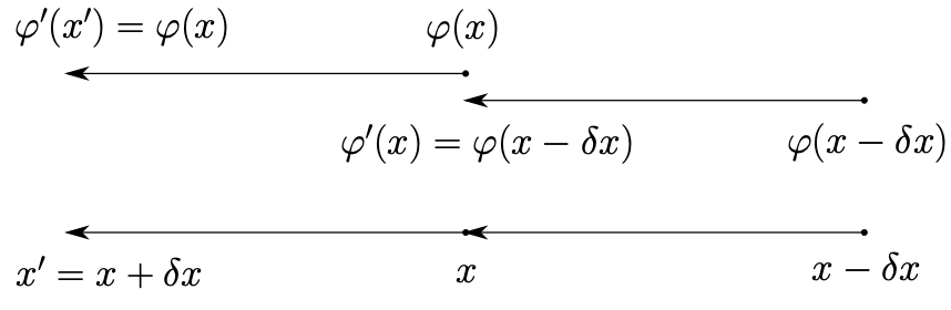
Scalar Field \(\varphi (x)\). We start with the questions how scalar fields \(\varphi (x)\) transform? For a scalar field, the value of the transformed field \(\varphi '\) at the transformed coordinate \(x'\) is the same as the field value before the transformation. \begin{equation} \varphi '(x') =\varphi (x). \label{eq:transformedscalarfield} \end{equation} We concentrate on an infinitesimal transformation and recall the transformation of the space-time vector \(x^\mu \): \begin{equation*} x'^{\mu } = \Lambda ^\mu _{~\nu }x^\nu ,\quad x'^{\mu } = x^\mu + \delta x^\mu , \quad \delta x^\mu =\delta \Lambda ^\mu _{\;\;\nu }x^\nu . \end{equation*} Since \(x-\delta x\) is transformed to \(x\) we find from eq. \eqref{eq:transformedscalarfield} the transformed field value \(\varphi '\) at the coordinate \(x\) \begin{equation*} \varphi '(x) = \varphi (x-\delta x). \end{equation*} We can visualise this by the picture shown in 1.
We want to consider field transformations at fixed coordinates and therefore employ \begin{equation*} \varphi '(x) = \varphi (x) + \delta \varphi (x) = \varphi (x-\delta x). \end{equation*} The transformation of \(\varphi \) at fixed \(x\) is called an active transformation, and we will employ this formulation. In contrast, leaving \(\varphi \) fixed and changing coordinates would be a passive transformation. (The combination of both does not change the field, \(\varphi '(x') = \varphi (x)\).)
The infinitesimal change of the field \(\delta \varphi \) at fixed coordinates obeys \begin{equation*} \begin{split} \delta \varphi = \varphi (x-\delta x) - \varphi (x)= -\partial _\mu \varphi (x)~\delta x^\mu . \end{split} \end{equation*} We assume here that \(\varphi (x)\) is a differentiable function, such that the second line reflects the definition of partial derivatives.
For Lorentz transformations we insert \(\delta x^\mu = \delta \Lambda ^\mu _{~\nu } x^\nu \) and find \begin{equation} \begin{split} \delta \varphi &= -\delta \Lambda ^\mu _{~\nu } x^\nu \partial _\mu \varphi (x)\\ &= -i\epsilon _z (T_z)^\mu _{~\nu }x^\nu \partial _\mu \varphi (x)\\ &= i \epsilon _z L_z\varphi (x). \end{split} \label{eq:deltaVarphi} \end{equation} For the last identity we have defined the generators for scalar fields \begin{equation*} L_z = -(T_z)^\mu _{\;\nu }x^\nu \partial _\mu . \end{equation*} The generators \(L_z\) contain a differential operator. Fields are infinite dimensional representations in a strict sense.
The letter \(L\) was not chosen arbitrary, as \(L_1\), \(L_2\) and \(L_3\) are the angular momenta. For instance \(L_1\) can be written as \begin{equation*} L_1 = -(T_1)^\mu _{~\nu } x^\nu \partial _\mu . \end{equation*} \(T_1\) has only two non-zero elements:\(\;(T_1)^2_{\;3} = -i\) and \((T_1)^3_{\;2} = i,\) implying \begin{equation*} \begin{split} L_1 &= -ix^2 \tfrac{\partial }{\partial x^3} + i x^3 \tfrac{\partial }{\partial x^2} = -i (y\partial _z - z\partial _y). \end{split} \end{equation*} Associating derivatives with momenta the three generators \(L_1\), \(L_2\) and \(L_3\) have the structure of angular momentum as we know it from classical mechanics: \(L = r ~\times ~ p\). In quantum mechanics, this is precisely the structure of the angular momentum operator. You may recall the commutation relation \([L_k,L_l]=i\epsilon _{klm}L_m\) which shows that we deal indeed with a representation of \(SO(3)\). Notice, however, that we have not used any operator formalism here. The generator \(L_z\) and their relations arise directly from the transformation properties of ”classical“ fields.
We conclude that the transformation of fields with Lorentz indices will have two ingredients. The first arises from the transformation of coordinates, the second is related to the Lorentz indices. For scalars one has only the coordinate part.
Vector Field \(A^\mu (x)\). Contravariant vectors transform as \begin{equation*} A^\mu (x) \quad \to \quad A'^{\mu }(x) = A^\mu (x) + \delta A^\mu (x), \end{equation*} where \begin{equation*} \delta A^\mu (x) = \delta \Lambda ^\mu _{\;\nu } A^\nu (x) + x^\rho \delta \Lambda _\rho ^{\;\sigma }\partial _\sigma A^\mu (x). \end{equation*} Here, \(\delta \Lambda ^\mu _{\;\nu }A^\nu \) is the usual transformation law for covariant vectors. The part \(x^\rho \delta \Lambda _\rho ^{\;\sigma }\partial _\sigma A^\mu \) reflects the change of the coordinates. It is the same as for scalar fields, using \begin{equation} x^\rho \delta \Lambda _\rho ^{\;\sigma }\partial _\sigma A^\mu =-\delta \Lambda ^\sigma _{\;\rho }x^\rho \partial _\sigma A^\mu , \label{eq:NN13} \end{equation} where we employ the antisymmetry of \(\delta \Lambda _{\sigma \rho }\). Since the Minkowski metric is Lorentz invariant the upper and lower positions of contracted indices can be exchanged, i.e. \(x^\rho \delta \Lambda _\rho ^{\;\sigma }=x_\rho \delta \Lambda ^{\rho \sigma }\), \(\delta \Lambda _\rho ^{\;\sigma } \partial _\sigma =\delta \Lambda _{\rho \sigma } \partial ^\sigma \) etc. The part arising from the transformation of coordinates is always the same, no matter what kind of field we are transforming.
Covariant vectors transform as: \begin{equation*} \delta A_\mu (x) = \delta \Lambda _\mu ^{\;\nu }A_\nu (x) + x^\rho \delta \Lambda _\rho ^{\;\sigma }\partial _\sigma A^\mu (x). \end{equation*} The covariant derivative transforms as \begin{equation*} \begin{split} &\partial _\mu \varphi (x) \quad \to \quad (\partial _\mu \varphi )'(x) = \partial _\mu (\varphi (x)+\delta \varphi (x)) = \partial _\mu \varphi (x) + \delta \partial _\mu \varphi (x). \end{split} \end{equation*} One infers \begin{equation*} \begin{split} \delta &\partial _\mu \varphi (x) = \partial _\mu \delta \varphi (x) = \partial _\mu (x^\rho \delta \Lambda _\rho ^{~\sigma }\partial _\sigma \varphi (x)) =\delta \Lambda _\mu ^{~\sigma }\partial _\sigma \varphi (x) + (x^\rho \delta \Lambda _\rho ^{~\sigma }\partial _\sigma )(\partial _\mu \varphi (x)). \end{split} \end{equation*} Thus \(\partial _\mu \varphi (x)\) indeed transforms as a covariant vector field. With a similar argument one finds that the contravariant derivative transforms as a contravariant vector field. This implies \begin{equation*} \delta (\partial ^\mu \varphi (x)\partial _\mu \varphi (x)) = (x^\rho \delta \Lambda _\rho ^{\;\sigma }\partial _\sigma )(\partial ^\mu \varphi (x) \partial _\mu \varphi (x)), \end{equation*} and \(\partial ^\mu \varphi (x)\partial _\mu \varphi (x)\) therefore transforms as a scalar field.
Our aim is the construction of a Lorentz-invariant action as the starting point of formulating the functional integral for a quantum field theory. This is a central piece of our lecture. With all the machinery we have developed it is almost trivial. Now our works pays off. The basic construction principle is that an invariant action obtains as a space-time integral over a quantity that transforms as a scalar field. This scalar field is typically a composite expression, as \(\partial ^\mu \varphi (x) \partial _\mu \varphi (x)\).
Let \(f(x)\) be some (composite) scalar field with infinitesimal Lorentz transformation \begin{equation*} \delta f = x^\rho \delta \Lambda _\rho ^{\;\sigma }\partial _\sigma f. \end{equation*} Examples constructed from scalar fields \(\varphi (x)\) are \(f= \varphi ^2\) or \(f= V(\varphi )\) or \(f= \partial ^\mu \varphi \partial _\mu \varphi \). It follows that an action constructed as \begin{equation*} S=\int d^4x ~f(x) \end{equation*} is Lorentz invariant, \(\delta S=0\). The proof of \(\delta S=0\) employs the vanishing of an integral over total derivatives, \begin{equation*} \begin{split} \delta S &= \int d^4x~ \delta f(x)= \int d^4x~ x^\rho \delta \Lambda _\rho ^{~\sigma }\partial _\sigma f\\ &= \int d^4 x~ \partial _\sigma (x^\rho \delta \Lambda _\rho ^{~\sigma }f) - \int d^4 x~ \delta ^\rho _\sigma \delta \Lambda _\rho ^{~\sigma }\partial _\sigma f= 0. \end{split} \end{equation*} More precisely, the first integral is zero because we always assume the absence of boundary contributions. Then total derivatives in \(\mathscr{L}\) can be neglected, \(\int d^4 x \partial _\mu A = 0.\) The second integral is zero because of the antisymmetry of \(\Lambda _{\rho \sigma }\): \begin{equation*} \delta ^\rho _\sigma \delta \Lambda _\rho ^{\;\sigma } = \eta ^{\rho \sigma }\delta \Lambda _{\rho \sigma } = 0. \end{equation*}
Examples.
It is now rather straight forward to construct possible actions for quantum field theories. Lorentz
invariant actions can be written as sums of invariant terms. \begin{equation*} S= \int d^4x \sum _k \mathscr{L}_k(x), \end{equation*}
where \(\mathscr{L}_k\) are (composite) scalar fields. Let us give some examples:
\begin{equation*} \mathscr{L} = \partial ^\mu \varphi ^*\partial _\mu \varphi + m^2 \varphi ^*\varphi . \end{equation*}
This is the action for a free charged scalar field. It describes particles with mass \(m\) like e.g. pions \(\pi ^{\pm }\) with
interactions neglected. \begin{equation*} \mathscr{L} = \tfrac{1}{4} F^{\mu \nu }F_{\mu \nu },\quad F_{\mu \nu } = \partial _\mu A_\nu - \partial _\nu A_\mu . \end{equation*}
This is the action for free photons. The antisymmetric tensor field \(F_{\mu \nu }(x)=-F_{\nu \mu }(x)\) is the electromagnetic field
strength. As in classical electrodynamics the components \(F_{0k}\) describe the electric field, while \(\epsilon _{ijk}F_{jk}\) denotes the
components of the magnetic field. \begin{equation*} \mathscr{L} = (\partial ^\mu + ie A^\mu )\varphi ^*(\partial _\mu -ie A_\mu )\varphi + \tfrac{1}{4} F^{\mu \nu }F_{\mu \nu }. \end{equation*}
This describes a charged scalar field interacting with photons. A model with the corresponding action is
called scalar QED where QED stands for quantum electrodynamics. The QED for electrons needs the
Lorentz invariant description of fermions in order to account for the spin of the electrons and
positrons.
9.6 Functional Integral, Correlation Functions
Measure and partition function. The partition function \(Z= \int D\varphi \; e^{-S}\) is invariant if the measure \(\int D\varphi \) and the action \(S\) are invariant. For a scalar field \(\varphi (x)\) the measure is indeed invariant \begin{equation*} \int D\varphi (x)=\int D\varphi '(x). \end{equation*} This follows from the equivalence of active and passive transformations, \begin{equation*} \varphi '(x) = \varphi (\Lambda ^{-1} x). \end{equation*} Since one integrates over \(\varphi \) at every point \(x\), this is equivalent to an integration at every point \(\Lambda ^{-1}x\). Similarly, for vectors one has \begin{equation*} \int DA^{\mu } = \int DA'^{\mu }\times \text{Jacobian}. \end{equation*} The Jacobian is a product over all \(x\) of factors \(\det \Lambda \). Since \(\det \Lambda =1\). The functional measure is again invariant.
Regularisation. The product over all positions is not always well defined. One typically aims for a regularisation, which defines the functional integral as some limiting process of finite-dimensional integrals, as we have done it in the beginning of this lecture. One possibility is a lattice regularisation, for which the continuous manifold of points is replaced by the sites of a lattice – typically \(a\) \(d\)-dimensional hypercubic lattice. This regularisation has the advantage that gauge symmetries can be implemented rather easily. A lattice of points does not admit continuous Lorentz transformations. For such a regularisation the functional measure is not Lorentz invariant. In this case one expects Lorentz invariance to show up only in the continuum limit for which the lattice distance gets very small as compared to all length scales of interest. Lorentz invariance of the continuum limit has to be proven. For the models that are investigated this is indeed realised. We will simply assume here that a Lorentz-invariant measure exists and use this property implicitly.
Correlation Function. For a Lorentz invariant action and measure the correlation functions have covariant transformation properties. For example, the correlation function \begin{equation*} \langle \varphi (x)\varphi (x')\rangle = Z^{-1} \int D\varphi \varphi (x) \varphi (x') e^{-S} \end{equation*} transforms in the same way as the product \(\varphi (x) \varphi (x')\). This covariant construction makes it easy to construct an invariant S-matrix. Then scattering cross sections and similar quantities are Lorentz invariant.
Summary. Explicit Lorentz covariance is an important advantage of the functional integral formulation of quantum field theories. In the operator formalism the implementation of Lorentz symmetry can sometimes be more complicated. The basic reason is that the operator formalism is a Hamiltonian formalism. The Hamiltonian is not Lorentz-invariant – it singles out a time direction. In contrast, the action is a four-dimensional object for which Lorentz invariance can be implemented in a very straightforward way.