
Quantum field theory 1, lecture 04
Periodic Boundary Condition. Replace \(\mathscr{L}_f+\mathscr{L}_\text{in}\) by \(-\beta s(x_\text{f})s(x_\text{in})\). This closes the circle by defining \(x_\text{f}\) and \(x_\text{in}\) as next neighbours. The partition function becomes \begin{equation*} Z= \text{Tr} \left \{\hat{T}^P \right \}. \end{equation*} Diagonalising \(\hat{T}\) solves the Ising model in a simple way, \begin{equation*} Z={\lambda _+}^P +{\lambda _-}^P, \end{equation*} with \(\lambda _{\pm }\) the two eigenvalues of the transfer matrix, \begin{equation*} \lambda _+ = 2\cosh (\beta ), \quad \quad \quad \lambda _- = 2\sinh (\beta ). \end{equation*} In the limit \(P \to \infty \) only the largest eigenvalue \(\lambda _+\) contributes.If we restore for \(\beta \) the product of coupling strength and inverse temperature, this is the exact solution for the canonical partition function for the Ising chain. The thermodynamics follows from there.
Generalisations. The transfer matrix can be generalised to an arbitrary number of Ising spins \(s_\gamma (x)\). For \(M\) spins, \(\gamma =1, \ldots ,M\), the transfer matrix \(\hat{T}\) is an \(N \times N\) matrix, \(N=2^M\), \(\tau =1,\ldots ,N\).
For example, if \(M=2\), \(\hat{T}\) is a \(4 \times 4\) matrix. The basis functions in the occupation number basis are taken as \begin{equation*} \begin{split} & h_1=n_1n_2, \quad \quad \quad \quad \quad \,\,\, h_2=(1-n_1)n_2,\\ & h_3=n_1(1-n_2), \quad \quad \quad h_4=(1-n_1)(1-n_2). \end{split} \end{equation*} This structure can be extended to arbitrary \(M\). The basis functions obey the same rules as discussed for \(M=1\). In particular, \(\gamma \) may denote a second coordinate \(y\) such that, \begin{equation*} s_\gamma (x)\to s(x,y). \end{equation*}
Two-dimensional Ising model. In this way one can define formally the transfer matrix for the two-dimensional Ising model. The coordinate \(x\) denotes now lines in a two-dimensional plane, see fig. 1.
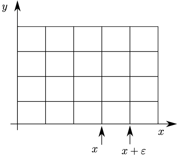
More generally, in \(d\) dimensions, \(x\) denotes the position on a particular \(d-1\) dimensional hypersurface. The transfer matrix contains the information of what happens if one goes from one hypersurface to the next one.
3.2 Non-commutativity in classical statistics
Local observables and operators. A local observable \(A(x)\) depends only on the local spin \(s(x)\). We want to find an expression for its expectation value in terms of the transfer matrix. For this purpose we consider the expression \begin{equation*} \sum _{s(x)}\mathscr{K}(x) A(x) \mathscr{K}(x-\varepsilon ) = \sum _{s(x)} h_\tau (x+\varepsilon )\hat{T}_{\tau \rho }(x)h_\rho (x)A_\gamma (x)h_\gamma (x)h_\alpha (x)\hat{T}_{\alpha \beta }(x-\varepsilon )h_\beta (x-\varepsilon ), \end{equation*} where we use the shorthand \begin{equation*} h_\tau (x)= h_\tau (s(x)), \end{equation*} and the expansion \begin{equation*} A(x) = A_\gamma (x) \, h_\gamma (s(x)). \end{equation*} We employ \begin{equation*} A_\gamma (x)\sum _{s(x)} h_\rho (x)h_\gamma (x)h_\alpha (x)=\sum _\gamma A_\gamma (x)\delta _{\rho \gamma }\delta _{\gamma \alpha }, \end{equation*} and introduce the diagonal operator \begin{equation*} (\hat{A}(x))_{\rho \alpha }=\sum _\gamma A_\gamma (x)\delta _{\rho \gamma }\delta _{\gamma \alpha }=\begin{pmatrix} A_1(x) & 0 \\ 0 & A_2(x) \end{pmatrix}. \end{equation*} The last identity refers to the single spin Ising chain. The two observables \(A_1\) and \(A_2\) correspond to the values that the observable takes in the two local states of the Ising chain. The fact that the operator is diagonal reflects properties of the specific occupation number basis. For a general basis the operator is not diagonal.
In terms of this operator we can write \begin{equation*} \sum _{s(x)}\mathscr{K}(x)A(x)\mathscr{K}(x-\varepsilon ) =h_\tau (x+\varepsilon )\hat{T}_{\tau \rho }(x)\hat{A}_{\rho \alpha }(x)\hat{T}_{\alpha \beta }(x-\varepsilon )h_\beta (x-\varepsilon ). \end{equation*} The expectation value of \(A(x)\) obtains by an insertion of the operator \(\hat{A}(x)\), \begin{equation*} \begin{split} \langle A(x) \rangle &= \frac{1}{Z}\int Ds \, e^{-S}A(x)\\ &=\frac{1}{Z} \bar{q}_\tau (x_\text{f})[\hat{T}(x_\text{f}-\varepsilon ) \cdots \hat{T}(x)\hat{A}(x)\hat{T}(x-\varepsilon ) \cdots \hat{T}(x_\text{in})]_{\tau \rho }\tilde{q}_\rho (x_\text{in}) \end{split} \end{equation*} The operators \(\hat{T}(x)\) and \(\hat{A}(x)\) do in general not commute, \begin{equation*} [\hat{T}(x),\hat{A}(x)]\neq 0. \end{equation*} Non-commutativity is present in classical statistics if one asks questions related to hypersurfaces!
Let us concentrate on observables that are represented by operators \(\hat{A}\) which are independent of \(x\). As an example we take the local occupation number \(n(x)=2s(x)-1\). The associated operator is \begin{equation*} \hat{N}=\begin{pmatrix} 1 & 0 \\ 0 & 0 \end{pmatrix}. \end{equation*} If we want to obtain the expectation value at \(x\), we need to compute \begin{equation*} \langle n(x) \rangle = \frac{1}{Z}\langle \bar{q_f} | \hat{T}(x_\text{f}-\varepsilon )\cdots \hat{T}(x)\hat{N}\hat{T}(x-\varepsilon )\cdots \hat{T}(x_\text{in})| \tilde{q}_\text{in}\rangle , \end{equation*} where we employ a notation familiar from quantum mechanics, \begin{equation*} \langle \bar{q}_\text{f} | \hat{M} | \tilde{q}_\text{in}\rangle = (\bar{q}_\text{f} (x_\text{f}))_\tau \hat{M}_{\tau \rho }(q_\text{in}(x_\text{in}))_\rho . \end{equation*} A normalisation with \(Z=1\) brings the expression even closer to quantum mechanics. We adopt it in the following.
We may next consider the operator \begin{equation} \hat{N}_+ = \hat{T}(x)^{-1}\, \hat{N}\, \hat{T}(x), \label{eq:Nplus} \end{equation} and compute \begin{equation*} \langle \bar q_\text{f} | \hat{T}(x_f-\varepsilon ) \cdots \hat{T}(x)\hat{N}_+\hat{T}(x-\varepsilon )\cdots \hat{T}(x_\text{in}) | \tilde q_\text{in}\rangle = \langle n(x+\varepsilon )\rangle . \end{equation*} When we use the same prescription (with \(x\) singled out as a reference point) the operator \(\hat{N}\) corresponds to the observable \(n(x)\), while \(\hat N_+\) is associated to the observable \(n(x+\varepsilon )\). The operator \(\hat{N_+}\) is not diagonal and does not commute with \(\hat{N},\) \begin{equation*} [\hat{N}_+,\hat{N}] \neq 0. \end{equation*} We conclude that non-commuting operators do not only appear in quantum mechanics. The appearance of non-commuting structures is an issue of what questions are asked and which formalism is appropriate for the answer to these questions. One can actually device a Heisenberg picture for classical statistical systems in close analogy to quantum mechanics. The Heisenberg operators depend on \(x\) and do not commute for different \(x\).
3.3 Classical Wave functions
We have seen how operators and non-commuting structures appear within classical probabilistic systems. The transfer matrix formalism is a type of Heisenberg picture for classical statistics. There is also a type of Schrödinger picture with wave functions as probability amplitudes. This will be discussed in the present lecture.
Local probabilities. We start from the ”overall probability distribution” given for the Ising chain by \begin{equation*} p[s]= \frac{1}{Z} e^{-S[s]}, \quad \quad \quad Z = \int Ds \, e^{-S[s]}. \end{equation*} A local probability distribution at \(x\), which involves only the spin \(s(x)\), can be obtained by summing over all spins at \(x'\neq x\), \begin{equation*} p_l(s(x)) = \frac{1}{Z} \left [\prod _{x'\neq x}\sum _{s(x')=\pm 1}\right ] e^{-S} \equiv p_l(x). \end{equation*} It is properly normalized, \begin{equation*} \sum _{s(x)=\pm 1} p_l(s(x)) =1. \end{equation*} The expectation value of the spin \(s(x)\) can be computed from \(p_l(s(x))\), \begin{equation*} \langle s(x) \rangle = \sum _{s(x)=\pm 1} p_l(s(x))s(x). \end{equation*} If there would be a simple evolution law how to compute \(p_l(x+\varepsilon )\) from \(p_l(x)\), one could solve the boundary value problem iteratively, starting from the initial probability distribution \(p_l(x_\text{in})\). The evolution law would permit us to infer \(p_l(x)\), and therefore to compute the expectation value of \(s(x)\). Unfortunately, such a simple evolution law does not exist for the local probabilities. We will see next that it exists for local wave functions or probability amplitudes.
Wave Functions. Define for a given \(x\) the partial actions \(S_-\) and \(S_+\) by \begin{equation*} \begin{split} S_- = & \mathscr{L}_{\text{in}}+\sum _{x^\prime =x_\text{in}}^{x-\varepsilon } \mathscr{L}(x^\prime ),\\ S_+ = & \sum _{x^\prime =x}^{x_\text{f}-\varepsilon } \mathscr{L}(x^\prime ) + \mathscr{L}_\text{f}, \\ S = & S_- + S_+. \end{split} \end{equation*} Here \(S_-\) depends only on the Ising spins \(s(x')\) with \(x'\leq x\), and \(S_+\) depends on spins \(s(x')\) with \(x'\geq x\).
The wave function \(f(x)\) is defined by \begin{equation*} f(x) = \left [\prod _{x^\prime =x_\text{in}}^{x-\varepsilon } \sum _{s(x^\prime )=\pm 1} \right ] e^{-S_-}. \end{equation*} Because we sum over all \(s(x^\prime )\) with \(x^\prime < x\), and \( S_-\) depends only on those \(s(x^\prime )\) and on \(s(x)\), the wave function \(f(x)\) depends only on the single spin \(s(x)\). Similarly, we define the conjugate wave function \begin{equation*} \bar{f}(x) = \left [ \prod _{x'=x+\varepsilon }^{x_f} \sum _{s(x')=\pm 1} \right ] e^{-S_+}, \end{equation*} which also depends only on \(s(x)\).
Wave functions and local probability distribution. The product \begin{equation*} \bar f(x) f(x)= \left [ \prod _{x' \neq x} \sum _{s(x')= \pm 1} \right ] e^{-S} = Z \, p_l(x), \end{equation*} is closely related to the local probability distribution \(p_l(x)\). One has \begin{equation*} \sum _{s(x)=\pm 1} \bar{f}(x)f(x) = Z. \end{equation*} In the following we employ the possibility of an additive renormalisation \( S\to S+C\) in order to normalise the partition function to \( Z=1\). This can be achieved by adding a constant to \(\mathscr{L}(x)\), and similarly for the boundary terms \(\mathscr{L}_\text{in}\) and \(\mathscr{L}_\text{f}\). With \(Z=1\) the wave functions \(\bar f\) and \(f\) are a type of probability amplitudes, similar as in quantum mechanics. We have, however, two distinct types of probability amplitudes, \(f\) and \(\bar{f}\).
Quantum rule for expectations values of local observables. The expectation value of a local observable \(A(x)\) can be written in terms of a bilinear in the wave functions. \begin{equation*} \begin{split} \langle A(x) \rangle &= \sum _{s(x)=\pm 1} A(x) p_l(x)\\ &= \frac{1}{Z} \sum _{s(x)=\pm 1} \bar{f}(x)A(x)f(x). \end{split} \end{equation*} We expand again in the occupation number basis \begin{equation*} \begin{split} &f(x) = \tilde{q}_\rho (x)h_\rho (x),\\ &\bar{f}(x)=\bar{q}_\tau (x)h_\tau (x),\\ &A(x)=A_\sigma (x)h_\sigma (x). \end{split} \end{equation*} Here \(\tilde{q}_\rho (x)\) are the components of the wave function in the occupation number basis at \(x\), and \(\bar{q}_\tau (x)\) are the components of the conjugate wave function. This yields for the expectation values \begin{equation*} \langle A(x) \rangle = \frac{1}{Z} \bar{q}_\tau (x)A_\sigma (x)\tilde q_\rho (x) \sum _{s(x)=\pm 1}h_\tau (x)h_\sigma (x)h_\rho (x). \end{equation*} Using again the product properties of the basis functions one finds the “quantum rule” for the expectation value as a bilinear in the wave functions, \begin{equation} \begin{split} \langle A(x) \rangle &= \frac{1}{Z} \langle \bar{q}(x) | \hat{A}(x) | \tilde q(x) \rangle \\ &= \frac{1}{Z} \sum _\sigma \bar{q}_\tau (x) A_\sigma (x) \delta _{\tau \sigma }\delta _{\sigma \rho }\tilde{q}_\rho (x). \end{split}\label{eq:Ax} \end{equation} Knowledge of the wave function at \(x\) is therefore sufficient for the computation of \(\langle A(x) \rangle \).
In particular, for \(Z=1\) the rule \eqref{eq:Ax} is very close to quantum mechanics, except that \(\tilde q\) and \(\bar q\) are real wave functions and \(\bar q\) is not related to \(\tilde q\). As in quantum mechanics, it associates an operator to an observable, and employs the concept of probability amplitudes. We can not only express the expectation values of local observables as \(n(x)\), represented by \(\hat N(x)\), in this way. The relation \eqref{eq:Ax} also holds for the observable \(n(x+\varepsilon )\), represented by the operator \(\hat N_+\) in equation \eqref{eq:Nplus}. The rule \eqref{eq:Ax} may be called the “quantum rule”. In contrast to quantum mechanics it is not a new postulate. It follows from the basic probabilistic definition of expectation values in classical statistics by an appropriate organization of the probabilistic information.
Evolution equation for the wave function. In contrast to the local probability distribution, the \(x\)-dependence of the wave functions is a simple linear evolution law. This makes the wave function the appropriate object for the discussion of boundary value problems and beyond. From the definition of the wave function \(f(x)\) one infers immediately \begin{equation*} f(x+\varepsilon ) = \sum _{s(x)=\pm 1} \mathscr{K}(x) f(x). \end{equation*} As it should be, \(f(x+\varepsilon )\) depends on the spin \(s(x+\varepsilon )\). The expansion in the occupation number basis yields \begin{equation*} \begin{split} f(x+\varepsilon ) &= \tilde q_\tau (x+\varepsilon ) h_\tau (x+\varepsilon )\\ &= \sum _{s(x)=\pm 1} h_\tau (x+\varepsilon ) \hat{T}_{\tau \rho }(x)h_\rho (x) \, \tilde q_\sigma (x)h_\sigma (x)\\ &=\hat{T}_{\tau \rho }(x)\tilde{q}_\rho (x)h_\tau (x+\varepsilon ). \end{split} \end{equation*} The linear evolution operator for the wave function is the transfer matrix. \begin{equation*} \tilde{q}_\tau (x+\varepsilon )= \hat{T}_{\tau \rho }(x)\tilde{q}_\rho (x), \end{equation*} or, in a vector matrix notation \begin{equation*} \tilde{q}(x+\varepsilon ) = \hat{T}(x) \tilde{q}(x). \end{equation*}
By the same type of argument one obtains for the conjugate wave function (as a row vector) \begin{equation*} \bar{q}(x) = \bar{q}(x+\varepsilon ) \hat{T}(x), \end{equation*} or, written as a column vector, \begin{equation*} \bar{q}(x) = \hat{T}^T(x) \bar{q}(x+\varepsilon ), \end{equation*} and \begin{equation*} \bar{q}(x+\varepsilon ) = (\hat{T}^T (x))^{-1} \bar{q}(x). \end{equation*} In cases where \(\hat{T}\) is orthogonal, \(\hat{T}^{-1} = \hat{T}^T\), both \(\bar{q}\) and \(\tilde{q}\) obey the same evolution law. The evolution law is linear. The superposition law familiar from quantum mechanics follows. If \(\tilde{q}_1(x)\) and \(\tilde{q}_2(x)\) are two solutions of the evolution equation, this also holds for linear combinations \(\alpha \tilde{q}_1(x) + \beta \tilde{q}_2(x)\).
Continuous evolution. For a sufficiently smooth wave function \(\tilde{q}(x)\) one defines the derivative \begin{equation*} \begin{split} \frac{\partial \tilde{q}}{\partial x} &= \frac{1}{2\varepsilon }(\tilde{q}(x+\varepsilon ) - \tilde{q}(x-\varepsilon ))\\ &=\frac{1}{2\varepsilon }(\hat{T}(x)- \hat{T}^{-1}(x-\varepsilon ))\tilde{q}(x). \end{split} \end{equation*} This yields the generalised Schrödinger equation \begin{equation*} \begin{split} \partial _x \tilde q = & \frac{\partial }{\partial x} \tilde q = W \tilde{q}, \\ W(x) = & \frac{1}{2\varepsilon } \left [ \hat{T}(x)-\hat{T}^{-1}(x-\varepsilon ) \right ]. \end{split} \end{equation*} For the same \(\mathscr{L}\) at every \(x\), both \(\hat{T}\) and \(W\) are independent of \(x\), \begin{equation*} W=\frac{1}{2\varepsilon } \left [ \hat{T}-\hat{T}^{-1} \right ]. \end{equation*}
Step evolution operator. An additive renormalization of the action corresponds to a multiplicative renormalization of the transfer matrix. The step evolution operator is the transfer matrix normalized such that the absolute value of the largest eigenvalue equals unity. As the name indicates, the step evolution operator plays the same role as the discrete evolution operator in quantum mechanics. For the Ising model, the step evolution operator is given by \begin{equation*} \hat{T} = \frac{1}{2\cosh (\beta )}\begin{pmatrix} e^\beta & e^{-\beta } \\ e^{-\beta } & e^{\beta } \end{pmatrix}. \end{equation*}
Equilibrium state. If only one eigenvalue of the step evolution operator equals unity in absolute magnitude, the eigenstate to this eigenvalue is the unique equilibrium state \(\tilde{q}_*\). For the Ising model the equilibrium wave function is \begin{equation*} \tilde{q}_* \sim \begin{pmatrix} 1 \\ 1 \end{pmatrix}. \end{equation*} The equilibrium state is invariant under the evolution.
Boundary value problem. For given boundary conditions \(\tilde{q}(x_\text{in})\) and \(\bar{q}(x_\text{f})\) are fixed. One can use the evolution equation to compute both \(\tilde{q}(x)\) and \(\bar{q}(x)\). The value of a local observable \(A(x)\), with associated operator \(\hat{A}(x)\), follows from \begin{equation*} \langle A(x) \rangle = \frac{1}{Z}\langle \bar{q}(x) | \hat{A}(x)| \tilde{q}(x) \rangle . \end{equation*} Choose for \(\tilde{q}(x_\text{in})\) a decomposition into eigenfunctions of the transfer matrix \(\hat{T}\), e. g. with eigenvalues \(\lambda _+\) and \(\lambda _-\), \begin{equation*} \tilde{q}(x_\text{in}) = c_+(x_\text{in}) \tilde{q}_+ + c_- (x_\text{in}) \tilde{q}_-, \end{equation*} such that \begin{equation*} \tilde{q}(x) = \tilde{q}(x_\text{in}+N \varepsilon ) = c_+(x_\text{in}) \, (\lambda _+)^N \, \tilde{q}_+ + c_-(x_\text{in}) \, (\lambda _-)^N \, \tilde{q}_- . \end{equation*} For \(\lambda _+ = 1\), the corresponding eigenfunction is the equilibrium wave function, \begin{equation*} \lambda _+^N \tilde{q}_+ = \tilde{q}_+. \end{equation*} For \(\lambda _- < 1\) the contribution \(\sim (\lambda _-)^N \tilde{q}_-\) vanishes for large \(N\). This describes the approach to equilibrium. The correlation length is directly related to \(\lambda _-\). Similar rules are valid for the conjugate wave function. For a finite distance from the boundary we can employ the two wave functions in order to compute the expectation value of \(s(x)\) in dependence on given boundary conditions.
Generalisations and summary. The discussion for the Ising chain with a single spin at each site is easily generalised to \(M\) spins at each site, to multi-dimensional Ising models and to arbitrary overall probability distributions. The main purpose of this lecture was to give you a basic understanding how the functional integral and the operator formalism of quantum mechanics are related. When we discuss later the functional integral for relativistic quantum field theories no basic new concepts need to be introduced for the translation to the still more familiar operator formalism that is the starting point of most textbooks.
All these properties point to a close connection between quantum mechanics and classical statistics. Indeed, quantum mechanics can be understood as a sub-field of classical statistics. Quantum systems are realized as appropriate subsystems of ”classical” probabilistic systems. This is not the topic of this lecture. If you are interested, you may read ”The probabilistic world” [arXiv:2011.02867].