
Quantum field theory 1, lecture 03
2.5 Classical statistical thermodynamics
Hamiltonian and partition function. We have now all the ingredients for a microscopic formulation of thermodynamics. The well-known macroscopic thermodynamic laws all follow from this microscopic formulation. Furthermore, the behaviour of particular systems is encoded in the partition function which yields the “equation of state” of a given system.
The starting point is the classical Hamiltonian \(H\) for a given model. It is a functional of the microscopic variables \(\phi \), \(H[\phi ]\). For our example of \(O(N)\)-models, these variables are the fields \(\phi _n(x)\), or for the non-linear \(\sigma \)-models (including the Ising model), the constrained fields \(\pi _n(x)\). The Hamiltonian associates to each field configuration an energy \(H[\phi ]\). The classical action reads \begin{equation*} S[\phi ] = \beta H[\phi ] = \frac{H[\phi ]}{T}, \end{equation*} with \(\beta =1/T\) the inverse temperature. The functional integral yields for vanishing source \(J=0\) the partition function \(Z(\beta )\). The mean energy is found as \begin{equation*} E = \langle H \rangle = - \frac{\partial \ln Z(\beta )}{\partial \beta }, \end{equation*} relating \(E\) to the temperature \(T\). In this simplest version \(Z(\beta )\) is the partition function of the canonical ensemble, and the entropy \(\tilde S\) is defined as \begin{equation*} \tilde S = \left (1-\beta \frac{\partial }{\partial \beta }\right ) \ln Z(\beta ). \end{equation*}
Particle number. In the case of systems with a preserved particle number \(N\) we can also include in the action a term \(-\beta \mu N[\phi ]\), with \(N[\phi ]\) the particle number and \(\mu \) the chemical potential, \begin{equation*} S = \beta H[\phi ] - \beta \mu N[\phi ]. \end{equation*} In this case the partition function \(Z(\beta , \mu )\) is the grand canonical partition function, with mean particle number \(N\), mean energy \(E\) and entropy \(\tilde S\) given by \begin{equation*} \begin{split} & N = \frac{1}{\beta } \frac{\partial }{\partial \mu } \ln Z(\beta , \mu ), \quad \quad E = - \frac{\partial }{\partial \beta } \ln Z(\beta , \mu ) + \mu N, \\ & \tilde S = \left (1 - \beta \frac{\partial }{\partial \beta } \right ) \ln Z(\beta , \mu ). \end{split} \end{equation*} All thermodynamic relations follow from this setting, and the particular form of the grand canonical potential or Gibbs free energy \(\Omega = - \ln Z(\beta , \mu ) / \beta \) yields the equation of state of the system.
Magnetization. Source terms such as a homogeneous magnetic field for the case where \(\phi _n(x)\) describes magnetization, can be added. If we take \(\vec \phi (x)\) to be a microscopic magnetization density and \(\vec B\) a constant magnetic field, the action becomes \begin{equation} S = \beta H[\phi ] - \beta \kappa \int _x \phi _n(x) B_n. \end{equation} The macroscopic magnetization \(\vec M\) as a function of \(\vec B\) and temperature \(T\) obtains from \(Z(\beta , \vec B)\) as \begin{equation*} M_n = \frac{T}{\kappa } \frac{\partial \ln Z}{\partial B_n}. \end{equation*}
Pressure. If one wants to investigate questions related to volume and pressure, one has to confine the system in a box with volume \(V\) with suitable, for example periodic, boundary conditions for \(\phi (x)\). The partition function depends in this case on \(V\) as an additional parameter, and the pressure \(p\) obeys \begin{equation*} p = \frac{1}{\beta } \frac{\partial }{\partial V} \ln Z(\beta , \mu , V). \end{equation*} The functional integral is an object that you should know well from your course on statistical physics.
3 Operators and transfer matrix
Our approach to quantum field theory will be based on the discussion of functional integrals. These are a generalization of ordinary, multi-dimensional integrals to the limit of infinitely many degrees of freedom, i. e. infinite dimensional integrals. For bosons, the variables or fields all commute. (For fermions we will later use the anti-commuting Grassmann variables). One has learned that non-commuting operators play a crucial role in quantum mechanics. These non-commuting structures are not immediately visible in the bosonic functional integral which on first sight only contains commuting quantities. One may wonder how such integrals can describe the non-commutative properties of quantum mechanics. In the following we want to reveal the structural relation between the operator formalism, known from quantum mechanics, and the functional integral.
3.1 Transfer matrix for the Ising model
Boundary problem for Ising chain. Let us consider the one-dimensional Ising model \begin{equation*} S =\sum _x \mathscr{L}(x) + \mathscr{L}_\text{in} + \mathscr{L}_\text{f}, \end{equation*} with a next-neighbor interaction \(\mathscr{L}(x) = -\beta s(x+\varepsilon ) s(x)\) and initial and final boundary terms \(\mathscr{L}_\text{in}\) and \(\mathscr{L}_\text{f}\). (We combine interaction strength and inverse temperature into a single dimensionless parameter \(\beta \).) We choose boundary conditions such that \(s(x_\text{in})=1\) and \(s(x_\text{f})= 1\). This can be implemented by \begin{equation*} e^{-\mathscr{L}_\text{in}}=\delta (s(x_\text{in})-1), \quad \quad \quad e^{-\mathscr{L}_{f}}=\delta (s(x_\text{f})-1), \end{equation*} which in turn can be implemented by limits like \begin{equation*} \mathscr{L}_\text{in}=-\lim _{\kappa \to \infty } \kappa [s(x_\text{in})-1]. \end{equation*}
The question arises now: What is the expectation value \(\langle s(x) \rangle \) for \(x\) in the bulk, i. e. between the endpoints \(x_\text{in}\) and \(x_\text{f}\) ? The single configuration with minimal action has all spins aligned, \({s(x)}=1\). There are, however, many more configurations where some of the spins take negative values. Even though the particular probability for one such configuration is smaller, this is outweighed by the number of configurations. Qualitatively one expects something like in figure 1.
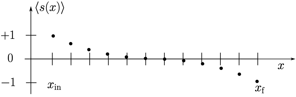
In the bulk, far away from the boundaries, the average spin may vanish to a good approximation. We look for a formalism to compute this behaviour as a function of the parameter \(\beta \).
Product form of probability distribution. We can write \(e^{-S}\) in product form \begin{equation*} e^{-S}= e^{-{\mathscr{L}_\text{f} + \sum _x \mathscr{L}(x) + \mathscr{L}_\text{in}}} = \bar{f}_\text{f} \left [\prod _x e^{-\mathscr{L}(x)}\right ]{f}_\text{in}= \bar{f}_\text{f}\left [ \prod _x \mathscr{K}(x) \right ]{f}_\text{in} \end{equation*} with boundary terms \(\bar{f}_\text{f}=e^{-\mathscr{L}_\text{f}}\) and \({f}_\text{in}=e^{-\mathscr{L}_\text{in}}\). Here \(\mathscr{K}(x)\) depends on the two spins \(s(x)\) and \(s(x+\varepsilon )\), while \( f_\text{in}\) depends on \(s(x_\text{in})\) and \(\bar f_\text{f}\) depends on \(s(x_\text{f})\).
Occupation number basis. Any function \(f(s(x))\) that depends only on the spin \(s(x)\) can be expanded in terms of two basis functions \(h_\tau (s(x))\) where \(\tau =1,2\), \begin{equation*} f(s(x)) = q_1(x) \, h_1(s(x)) + q_2(x) \, h_2(s(x)). \end{equation*} We choose the occupation number basis with \begin{equation*} h_1(s)=\frac{1+s}{2} = n, \quad \quad \quad h_2(s)=\frac{1-s}{2} = (1-n). \end{equation*} This is easily seen by noting that the occupation number \(n\) has only the values \(1\) (for \(s=1\)) and 0 (for \(s=-1\)), such that \begin{equation*} n^2=n. \end{equation*} Any polynomial in \(s\) can be written as \(an+b\), such that any \(f(s)\) can indeed be expressed in terms of the two basis functions.
We note some properties of the basis functions. The relation \begin{equation*} h_\tau (s) h_\rho (s) = \delta _{\tau \rho }h_\rho (s) \end{equation*} is simply verified by \(h_\tau ^2(s) = h_\tau (s)\) and \(h_1(s) h_2(s) = 0\)). Other useful relations are \begin{equation*} \sum _{s=\pm 1} h_\tau (s) = h_\tau (s=1) + h_\tau (s=-1)=1, \end{equation*} \begin{equation*} \sum _\tau h_\tau (s) = h_1(s) + h_2(s) =1, \end{equation*} and finally by combination \begin{equation*} \sum _{s=\pm 1} h_\tau (s) h_\rho (s) = \delta _{\tau \rho }. \end{equation*}
Transfer matrix. Let us now expand \(\mathscr{K}(x)\) in terms of the basis functions \(h_\tau (s(x+\varepsilon ))\) and \(h_\rho (s(x))\), \begin{equation*} \mathscr{K}(x) = \hat{T}_{\tau \rho }(x) \, h_\tau (s(x+\varepsilon )) \, h_\rho (s(x)). \end{equation*} We use here the Einstein summation convention which implies summation over the indices \(\tau \) and \(\rho \). The expansion coefficients \(\hat{T}_{\tau \rho }(x)\) are the elements of the transfer matrix \(\hat{T}\). This is a \(2\times 2\) matrix. Indeed using shorthands \(\bar{n} = n(t+\varepsilon )\), \(n= n(t)\) and similar for \(\bar{h}_\tau \), \(h_\tau \), an arbitrary \(\mathscr{K}(x)\) can be written as \begin{equation*} \begin{split} \mathscr{K} &= a\bar{n} n + b\bar{n}+cn + d \\ &= \hat{T}_{11} \bar{h}_1 h_1 + \hat{T}_{12} \bar{h}_1 h_2 + \hat{T}_{21}\bar{h}_2 h_1 + \hat{T}_{22}\bar{h}_2 h_2. \end{split} \end{equation*}
Matrix product for transfer matrix. Consider now the product of two neighbouring factors \(\mathscr{K}(x+\varepsilon )\) and \(\mathscr{K}(x),\) summed over the common spin \(s(x+\varepsilon )\) \begin{equation*} \begin{split} \sum _{s(x+\varepsilon )} \mathscr{K}(x+\varepsilon ) \mathscr{K}(x) & = \sum _{s(x+\varepsilon )} h_\tau (s(x+2\varepsilon )) \hat{T}_{\tau \rho } (x+\varepsilon )) h_\rho (s(x+\varepsilon )) h_\alpha (s(x+\varepsilon )) \hat{T}_{\alpha \beta }(x) h_\beta (s(x)) \\ & =\sum _\rho \sum _{s(x+\varepsilon )} h_\tau (s(x+2\varepsilon )) \hat{T}_{\tau \rho }(x+\varepsilon ) \hat{T}_{\rho \beta }(x) h_\rho (s(x+\varepsilon )) h_\beta (s(x))\\ & = \sum _\rho h_\tau (s(x+2\varepsilon ))\hat{T}_{\tau \rho }(x+\varepsilon )\hat{T}_{\rho \beta }(x)h_\beta (s(x))\\ & = h_\tau (s(x+2\varepsilon ))\left [\hat{T}(x+\varepsilon )\hat{T}(x)\right ]_{\tau \beta } h_\beta (s(x)).\\ \end{split} \end{equation*} The second line uses \(h_\tau h_\rho = \delta _{\tau \rho } h_\rho \) and the third line \(\sum _s h_\rho = 1\). We observe that the matrix product of transfer matrices appears in this product. For the Ising model the factors \(\mathscr{K}(x)\) are the same for all \(x\) (except for different spins being involved), and therefore \(\hat{T}\) is independent of \(x\). One simply finds \begin{equation*} \sum _{s(x+\varepsilon )}\mathscr{K}(x+\varepsilon )\mathscr{K}(x) =h_\tau (s(x+2\varepsilon )){\left [\hat{T}^2\right ]}_{\tau \rho }h_\rho (s(x)). \end{equation*} Doing one more similar step yields \begin{equation*} \sum _{s(x+2\varepsilon )}\sum _{s(x+\varepsilon )} \mathscr{K}(x+2\varepsilon ) \mathscr{K}(x+\varepsilon ) \mathscr{K}(x)= h_\tau (s(x+3\varepsilon ))\left [\hat{T}(x+2\varepsilon ) \hat{T}(x+\varepsilon )\hat{T}(x)\right ]_{\tau \rho } h_\rho (s(x)), \end{equation*} and so on.
Partition function as product of transfer matrices. One can write the partition function as \begin{equation*} \begin{split} Z &= \left [\prod _{x=x_\text{in}}^{x_\text{f}}\sum _{s(x)} \right ]\bar{f}_\text{f}(s(x_\text{f})) \left [\prod _{x=x_\text{in}}^{(x_\text{f}-\varepsilon )}\mathscr{K}(x)\right ] f_\text{in}(s(x_{\text{in}}))\\ & = \sum _{s(x_\text{f})}\sum _{s(x_\text{in})} \bar f_\text{f}(s(x_\text{f}))\, h_\tau (s(x_\text{f}))\left [\hat{T}(x_\text{f}-\varepsilon )\cdots \hat{T}(x_\text{in})\right ]_{\tau \rho } h_\rho (s(x_\text{in})) f_\text{in}(s(x_\text{in}))\\ &= \sum _{s(x_\text{f})}\sum _{s(x_\text{in})} \bar{q}_\beta (x_\text{f}) \, h_\beta (s(x_\text{f})) \, h_\tau (s(x_\text{f}))\left [\hat{T}\cdots \hat{T}\right ]_{\tau \rho } h_\rho (s(x_\text{in})) \, \tilde{q}_\alpha (s(x_\text{in})) \, h_\alpha (s(x_\text{in})). \end{split} \end{equation*} Here we have expanded \(\bar f_\text{f}\) and \(f_\text{in}\) in terms of the basis functions, \begin{equation*} \begin{split} \bar{f}_\text{f}(s(x_\text{f})) =& \bar{q}_\beta (x_\text{f}) \, h_\beta (s(x_\text{f})), \\ f_\text{in}(s(x_\text{in})) = & \tilde{q}_\alpha (x_\text{in}) \, h_\alpha (s(x_\text{in})). \end{split} \nonumber \end{equation*} Performing the sums over the initial and final spins leads to \begin{equation*} Z= \bar{q}_\tau (x_\text{f}) \left [\hat{T}(x_\text{f}-\varepsilon ) \cdots \hat{T}(x_\text{in}) \right ]_{\tau \rho }\tilde{q}_\rho (x_\text{in}). \end{equation*} This has the structure of an initial vector (or wave function) \(\tilde{q}(x_\text{in})\) multiplied by a matrix, and then contracted with a final vector (or conjugate wave function) \(\bar{q}(x_\text{f})\). We can use the bracket notation familiar from quantum mechanics, \begin{equation*} Z = \langle \bar{q}(x_\text{f})| \hat{T}(x_\text{f}-\varepsilon )\cdots \hat{T}(x_\text{in})|\tilde{q}(x_\text{in})\rangle . \end{equation*}
This product formulae resembles quantum mechanics if one associates the transfer matrix with the infinitesimal evolution operator \(U(t)\) \begin{equation*} \psi (t+\varepsilon )=U(t)\psi (t), \end{equation*} where \begin{equation*} U(t)=e^{i\varepsilon H(t)}. \end{equation*} With \begin{equation*} \psi (t_\text{f})=U(t_\text{f}-\varepsilon )\cdots U(t_\text{in}) \psi (t_\text{in}), \end{equation*} one can write the transition amplitude in the form \begin{equation*} \langle \phi (t_\text{f})| \psi (t_\text{f})\rangle = \langle \phi (t_\text{f}) U(t_\text{f}-\varepsilon ) \cdots U(t_\text{in})| \psi (t_\text{in}) \rangle . \end{equation*} Formally, the map between quantum mechanics and the classical statistics of the Ising model is
| Quantum mechanics | Classical statistics |
| \(U \) | \(\hat T\) |
| \( t \) | \( x \) |
| \( \psi \) | \( \tilde q \) |
| \( \bar \phi \) | \( \bar q \) |
A main difference to quantum mechanics is that \(\hat{T}\) does not preserve the norm of the wave function.
Computation of the transfer matrix. Let us compute the transfer matrix for the Ising model. We employ the defining relation of the transfer matrix by an expansion of the local factor in terms of basis functions, \begin{equation*} e^{\beta \bar{s}s} = \hat{T}_{\tau \rho } \, h_\tau (\bar{s})\, h_{\rho }(s), \end{equation*} where we use the shorthand notation \begin{equation*} \bar{s}=s(x+\varepsilon ), \quad \quad \quad s=s(x). \end{equation*} Using the decomposition \begin{equation*} s = h_1 - h_2 = n-(1-n) = 2n-1, \end{equation*} and \begin{equation*} \beta \bar{s}s= \beta (\bar{h_1}-\bar{h_2})(h_1-h_2)= \beta (\bar{h}_1h_1+\bar{h}_2h_2-\bar{h}_1h_2-\bar{h}_2h_1), \end{equation*} one obtains by analyzing the four configurations of neighboring spins \((\bar s, s)\), \begin{equation*} e^{\beta \bar{s}s} =e^\beta (\bar{h}_1h_1+\bar{h}_2h_2)+ e^{-\beta }(\bar{h}_1 h_2 + \bar{h}_2 h_1). \end{equation*} From this one can read off the transfer matrix \begin{equation*} \hat{T}= \begin{pmatrix} e^\beta & e^{-\beta } \\ e^{-\beta } & e^\beta \end{pmatrix}. \end{equation*} In general the transfer matrix \(\hat{T}\) is not a unitary matrix as for quantum mechanics. For the Ising model \(\hat{T}(x)\) does not depend on \(x\) so that one obtains \begin{equation*} Z =\bar{q}_\tau (x_\text{f})\left [\hat{T}^{P-1}\right ]_{\tau \rho }\tilde{q}_\rho (x_\text{in}). \end{equation*}
Periodic Boundary Condition. Replace \(\mathscr{L}_f+\mathscr{L}_\text{in}\) by \(-\beta s(x_\text{f})s(x_\text{in})\). This closes the circle by defining \(x_\text{f}\) and \(x_\text{in}\) as next neighbours. The partition function becomes \begin{equation*} Z= \text{Tr} \left \{\hat{T}^P \right \}. \end{equation*} Diagonalising \(\hat{T}\) solves the Ising model in a simple way, \begin{equation*} Z={\lambda _+}^P +{\lambda _-}^P, \end{equation*} with \(\lambda _{\pm }\) the two eigenvalues of the transfer matrix, \begin{equation*} \lambda _+ = 2\cosh (\beta ), \quad \quad \quad \lambda _- = 2\sinh (\beta ). \end{equation*} In the limit \(P \to \infty \) only the largest eigenvalue \(\lambda _+\) contributes.If we restore for \(\beta \) the product of coupling strength and inverse temperature, this is the exact solution for the canonical partition function for the Ising chain. The thermodynamics follows from there.