Quantum field theory 1, lecture 22
10.4 Feynman rules and Feynman diagrams
Action and partition function. We are now ready to formulate the Feynman rules for a perturbative treatment of quantum electrodynamics. The microscopic action is \begin{equation*} \begin{split} S &= \int d^4 x \left \{-\frac{1}{4} F^{\mu \nu }F_{\mu \nu } - i\bar{\psi }\gamma ^\mu (\partial _\mu - ieA_\mu )\psi - im\bar{\psi }\psi \right \}\\ &= S_2[\bar{\psi },\psi , A]- \int d^4 x \; e \bar{\psi }\gamma ^\mu A_\mu \psi . \end{split} \end{equation*} The last term is cubic in the fields \(\bar{\psi },\psi \) and \(A_\mu \), while all others terms are quadratic. We will perform a perturbative expansion in the electric charge \(e\).
Let us write the partition function as \begin{equation*} Z[\bar{\eta },\eta ,J] = \int D\bar{\psi } D\psi DA \; \exp \left [iS[\bar{\psi },\psi ,A]+ i\int \left \{\bar{\eta }\psi +\bar{\psi }\eta +J^\mu A_\mu \right \} \right ] \end{equation*} with \(\bar{\eta }\psi = \bar{\eta }_\alpha \psi _\alpha \) where \(\alpha = 1, \ldots , 4\) sums over spinor components. Formally, one can write \begin{equation*} Z[\bar{\eta },\eta ,J] = \text{exp} \left [-e \int d^4 x \left (\frac{1}{i}\frac{\delta }{\delta J^\mu (x)}\right )\left (i\frac{\delta }{\delta \eta _\alpha (x)}\right )(\gamma ^\mu )_{\alpha \beta }\left (\frac{1}{i}\frac{\delta }{\delta \bar{\eta }_\beta (x)} \right )\right ] Z_2[\bar{\eta },\eta ,J], \end{equation*} with quadratic partition function \begin{equation*} \begin{split} Z_2 &= \int D\bar{\psi } D\psi DA \; \exp \left [iS_2[\bar{\psi },\psi ,A] + i\int \left \{\bar{\eta }\psi +\bar{\psi }\eta +J^\mu A_\mu \right \} \right ]\\ &= \exp \left [i \int d^4 x d^4 y \; \bar{\eta }(x) S(x-y) \eta (y) \right ] \\ & \;\; \times \exp \left [{\frac{i}{2}\int d^4 x d^4 y \; J^\mu (x) \Delta _{\mu \nu }(x-y) J^\nu (y)}\right ]. \end{split} \end{equation*}
Propagator for Dirac fermions. We have introduced here also the propagator for Dirac fermions, which is in fact a matrix in spinor space, \begin{equation*} \begin{split} S_{\alpha \beta }(x-y) &= -i \int \frac{d^4 p}{(2\pi )^4} \;e^{ip(x-y)} (ip_\mu \gamma ^\mu +m \mathbb{1})^{-1}_{\alpha \beta }\\ &= -i \int \frac{d^4 p}{(2\pi )^4} \; e^{ip(x-y)} \frac{(-i p_\mu \gamma^\mu + m\mathbb{1})_{\alpha \beta }}{p^2 + m^2 -i\epsilon }. \end{split} \end{equation*} We can now calculate S-matrix elements by first expressing them as correlation functions which get then evaluated in a perturbative expansion of the functional integral. These perturbative expressions have an intuitive graphical representation as we have briefly discussed before. We concentrate here on tree diagrams for which renormalization is not needed yet.
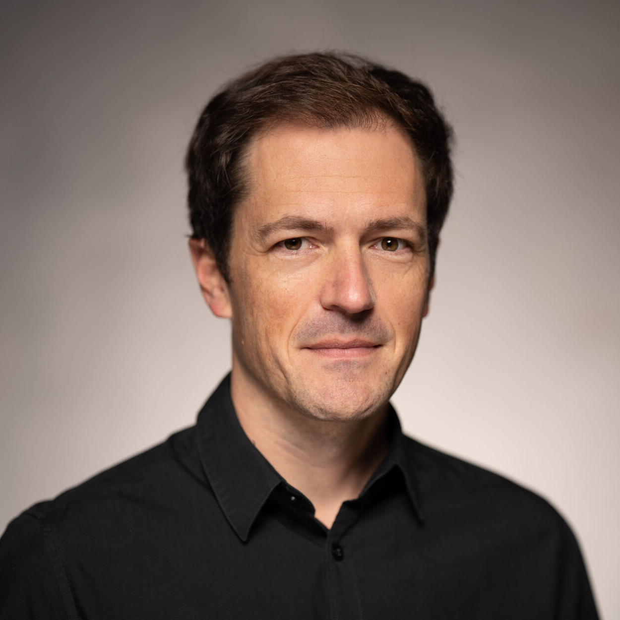
The correlation function of two Dirac fields can also be expressed in terms of the Dirac propagator, \begin{equation*} \langle \psi _\alpha (x) \bar{\psi }_\beta (y) \rangle = \frac{1}{Z_2}\left ( \frac{1}{i} \frac{\delta }{\delta \bar{\eta }_\alpha (x)}\right ) \left (i \frac{\delta }{\delta \eta _\beta (y)}\right ) Z_2{\Big |}_{\bar{\eta }=\eta =J=0} = \frac{1}{i} S_{\alpha \beta }(x-y). \end{equation*} We introduce a graphical representation for thus, as well,
 \((y, \beta) = \frac{1}{i} S_{\alpha \beta }(x-y).\)
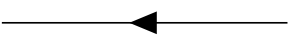
With sources \(i\bar{\eta }_\alpha (x)\) and \(i\eta _\beta (y)\) at the end this would be
 \( = \int _{x,y} i\bar{\eta }_\alpha (x) \; \frac{1}{i} S_{\alpha \beta }(x-y) \; i \eta _\beta (y) \)
\( = i\int _{x,y} \bar{\eta }(x) S(x-y) \eta (y). \)
\( = \int _{x,y} i\bar{\eta }_\alpha (x) \; \frac{1}{i} S_{\alpha \beta }(x-y) \; i \eta _\beta (y) \)
\( = i\int _{x,y} \bar{\eta }(x) S(x-y) \eta (y). \)
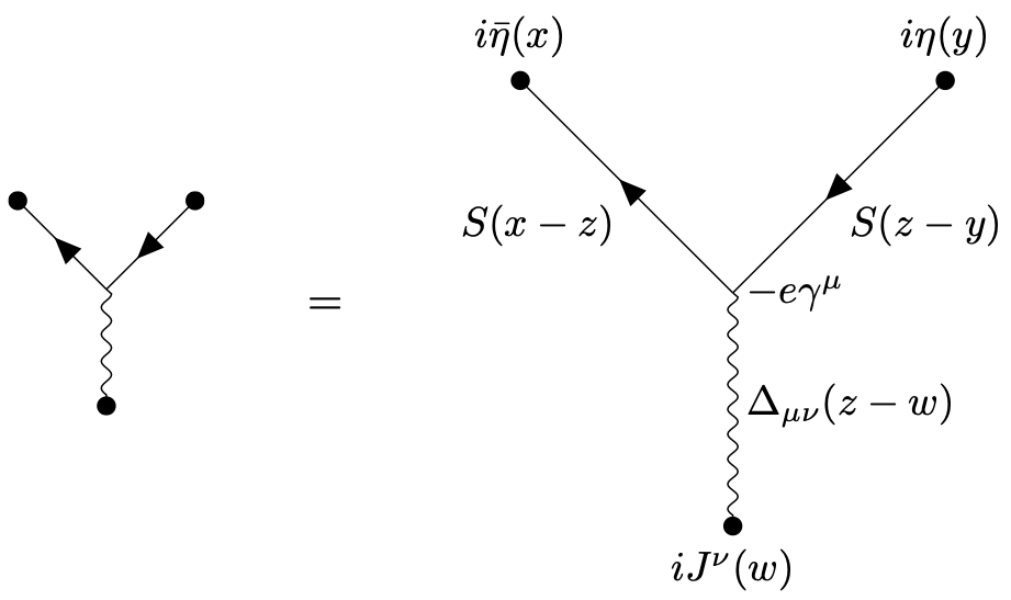
The conventions are such that the arrow points away from the source \(\eta \) and to the source \(\bar{\eta }\). It can also be seen as denoting the direction of fermions while anti-fermions move against the arrow direction. The Dirac indices \(\alpha ,\beta \) are sometimes left implicit when there is no doubt about them.
Expanding out exponentials. We now consider the full partition function and expand out the exponentials, \begin{equation*} \begin{split} Z[\bar{\eta },\eta ,J] = & \sum ^{\infty }_{V=0} \frac{1}{V!} \left [\int _x\left (\frac{1}{i}\frac{\delta }{\delta J^\mu (x)}\right ) \left (i\frac{\delta }{\delta \eta _\alpha (x)}\right )\left (-e\gamma ^\mu _{\alpha \beta }\right )\left (\frac{1}{i}\frac{\delta }{\delta \bar{\eta }_{\beta (x)}}\right )\right ]^V \\ &\times \sum ^{\infty }_{F=0} \frac{1}{F!}\left [\int _{x',y'} i\bar{\eta }_\alpha (x') \left (\frac{1}{i}S_{\alpha \beta }(x'-y') \right ) i\eta _{\beta }(y') \right ]^F\\ &\times \sum ^{\infty }_{p=0}\frac{1}{P!}\left [\frac{1}{2} \int _{x^{\prime \prime },y^{\prime \prime }} iJ^\mu (x^{\prime \prime }) \left (\frac{1}{i}\Delta _{\mu \nu }(x^{\prime \prime }-y^{\prime \prime }) \right ) iJ^\nu (y^{\prime \prime })\right ]^P. \end{split} \end{equation*} The index \(F\) counts the number of fermion propagators (corresponding to fermion lines in a graphical representation), the index \(P\) counts the number of photon propagators (photon lines). The index \(V\) counts vertices that connect fermion and photon in a specific way. More specifically, each power of this term removes one of each kind of sources and introduces \(-e\gamma ^\mu _{\alpha \beta }\) to connect the lines in the graphical representation.
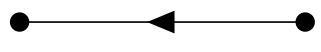
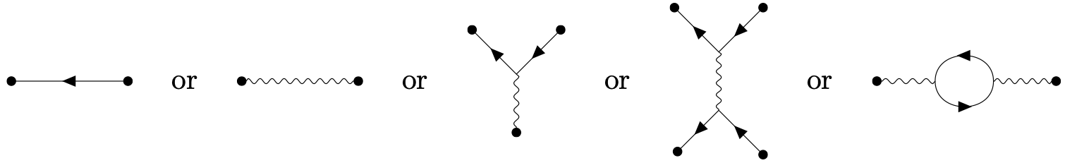
Graphical representation for partition function. In the full expression for \(Z[\bar \eta ,\eta ,J]\) many terms are present, in fact all graphs one can construct with fermion lines, photon lines and the vertex. For example
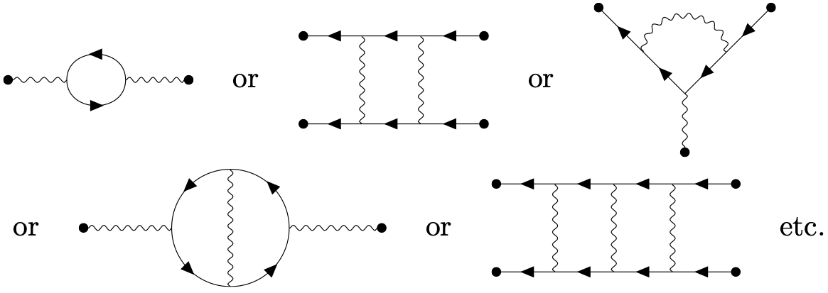
Connected and disconnected diagrams. One distinguishes connected diagrams where all endpoints are connected with lines to each other, for example
Disconnected diagrams can be decomposed into several connected diagrams.
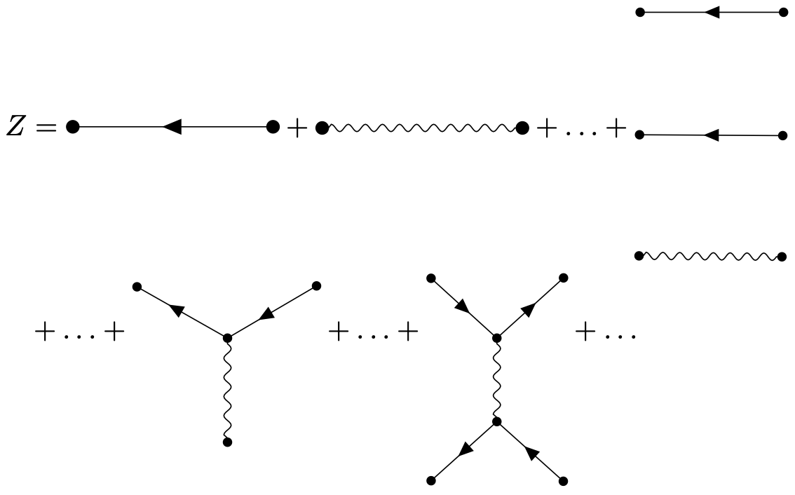
Tree and loop diagrams. One also distinguishes tree diagrams and loop diagrams. Loop diagrams have closed loops of particle flow, for example
Tree diagrams have no closed loop, for example
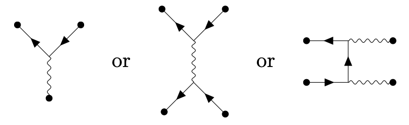
Corresponding algebraic expressions. To each of these diagrams with sources one can associate an expression, for example
To calculate S-matrix elements we are mainly interested in the connected diagrams because disconnected diagrams describe events where not all particles scatter. Also, we concentrate here on tree diagrams. Loop diagrams will be discussed somewhat later.
S-matrix elements. Now that we have seen how to represent \(Z[\bar{\eta },\eta , J],\) let us discuss how to obtain S-matrix elements. For example, for an outgoing photon we had the LSZ rule \begin{equation*} \sqrt{2E_p}\;a_{\vec{p},\lambda }(\infty ) \to i\epsilon ^{\nu *}_{(\lambda )}(p) \int d^4 x \; e^{-ipx} \left [-\partial _\mu \partial ^\mu \right ]A_\nu (x). \end{equation*} To obtain the field \(A_\nu (x)\) under the functional integral we can use \begin{equation*} A_\nu (x) \to \frac{1}{i} \frac{\delta }{\delta J^\nu (x)}, \end{equation*} acting on \(Z[\bar{\eta },\eta , J].\) Moreover, \(i[-\partial _\mu \partial ^\mu ]\) will remove one propagator line for the outgoing photon, \begin{equation*} \begin{split} & i\left [-\partial _\mu \partial ^\mu \right ] \frac{1}{i} \Delta _{\rho \sigma }(x-y) = \left [-\partial _\mu \partial ^\mu \right ]\int \frac{d^4p}{(2\pi )^4} e^{ip(x-y)} \frac{\mathscr{P}_{\rho \sigma }(p)}{p^2 - i\epsilon } \\ & =\int \frac{d^4 p}{(2\pi )^4} e^{ip(x-y)} \mathscr{P}_{\rho \sigma }(p) \to \eta _{\rho \sigma } \delta ^{(4)} (x-y). \end{split} \end{equation*} The projector has no effect if the photon couples to conserved currents and the result is simply \(\eta _{\rho \sigma } \delta ^{(4)} (x-y)\). What remains is to multiply with the polarization vector \begin{equation*} \epsilon ^{*}_{(\lambda )\mu }(p) \end{equation*} for the out-going photon with momentum \(p\). Also, the Fourier transform brings the expression to momentum space. The out-going momentum is on-shell, i. e. it satisfies \(p_\mu p^\mu =0\) for photons. Similarly, for incoming photons we need to remove the external propagator line and contract with \begin{equation*} \epsilon _{(\lambda )\mu }(p), \end{equation*} instead.
For out-going electrons we need to remove the external fermion propagator and multiply with \(\bar{u}_s(\vec{p})\) where p is the momentum of the out-going electron satisfying \(p^2 + m^2 =0\) and \(s\) labels its spin state. Similarly, for an incoming electron we need to contract with \(iu_s(p)\).
For out-going positrons we need to contract with \(iv_s(p)\) (and include here one factor \(i\) because \(i\bar{\psi }\) appears in the LSZ rule in our conventions). For an incoming positron the corresponding external spinor is \(\bar{v}_s(p)\).
Propagators in momentum space. Working now directly in momentum space, the photon propagator is represented by \begin{equation*} -i\frac{\mathscr{P}_{\mu \nu }(p)}{p^2 -i\epsilon } = -i \frac{\eta _{\mu \nu }-\frac{p_\mu \;p_\nu }{p^2}}{p^2-i\epsilon }. \end{equation*} The fermion propagator is \begin{equation*} -i\frac{-ip_\mu \gamma^\mu+m}{p^2+m^2-i\epsilon }. \end{equation*} The vertex is as before \(-e\gamma ^\mu \). Momentum conservation must be imposed at each vertex. Together these rules constitute the Feynman rules of QED. One can work with the graphical representation and then translate to formula at a convenient point. However, when in doubt, one can always go back to the functional representation.