Quantum field theory 1, lecture 23
10.5 Elementary scattering processes
We are now ready to use the formalism of quantum field theory, specifically quantum electrodynamics, to determine actually scattering amplitudes and cross section. The incoming and outgoing states can consist of photons, electrons and positrons but also muons or anti-muons and more generally any charged particles. When the charged particles are scalar bosons, one would use a variant of the theory called scalar electrodynamics, but we are here concerned with charged spin-\(1/2\) particles which are described by standard spinor electrodynamics.
In the following we will bring together several of the elements we have discussed before, such as
- the Lagrangian of spinor quantum electrodynamics,
- the idea of perturbation theory as an expansion in the coupling constant \(e\),
- the graphical representation in terms of Feynman diagrams,
- solutions to the free Dirac equation for incoming or outgoing electrons and positrons (or muons and anti-muons),
- the propagators for Dirac femions and for photons,
It might be a good idea to go back and revise these topics if you feel uncertain about them. We will see on the way that we need some additional technical knowledge, specifically
- how to do spin sums,
- how to calculate traces of gamma matrices
- how Mandelstam variables are defined and how one can work with them.
These points will also be discussed in the exercises.
We will then start to look at the elastic scattering of a photon and an electron, a process known as Compton scattering. We will write down the Feynman diagrams and the corresponding algebraic expressions. For another process, namely the scattering of an electron-positron pair to a muon-anti-muon pair we will do this, as well, but then also go on and evaluate the expressions further until we arrive at a nice and compact result for the scattering cross-section.
Compton Scattering. As a first example let us consider Compton scattering \(e^{-} \gamma \to e^{-} \gamma \)
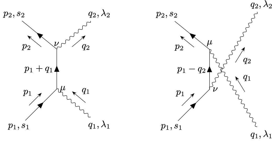
These are two diagrams at order \(e^2\), as shown above. The first diagram corresponds to the expression \begin{equation*} \bar{u}_{s_2}(p_2) (-e\gamma ^\nu )\left (-i\frac{-i(p_1 \cdot \gamma + q_1 \cdot \gamma)+m}{(p_1 + q_1)^2+m^2}\right )(-e\gamma ^\mu ) \; iu_s(p_1) \; \epsilon _{(\lambda _1)\mu } (q_1)\;\epsilon ^{*}_{(\lambda _2)\nu }(q_2) . \end{equation*} Similarly, the second diagram gives \begin{equation*} \bar{u}_{s_2}(p_2) (-e\gamma ^\mu )\left (-i\frac{-i(p_1 \cdot \gamma - q_1 \cdot \gamma )+m}{(p_1 - q_1)^2+m^2}\right )(-e\gamma ^\nu ) \; iu_s(p_1) \; \epsilon _{(\lambda _1)_\mu } (q_1)\;\epsilon ^{*}_{(\lambda _2)\nu }(q_2) . \end{equation*} Combining terms and simplifying a bit leads to \begin{equation*} i\mathcal{T} = e^2 \epsilon _{(\lambda _1)\mu }(q_1)\;\epsilon ^{*}_{(\lambda _2)\nu } (q_2) \; \bar{u}_{s_2}(p_2) \left [\gamma ^\nu \; \frac{-i(p_1 \cdot \gamma+ q_1 \cdot \gamma)+m}{(p_1+q_1)^2+m^2}\gamma ^\mu + \gamma ^\mu \frac{-i(p_1 \cdot \gamma-q_2 \cdot \gamma)+m}{(p_1 -q_2)^2+m^2}\gamma ^\nu \right ]u_{s_1}(p_1). \end{equation*}
Electron-positron to muon-anti-muon scattering. As another example for an interesting process in QED we consider \(e^{-} e^{+} \to \mu ^{-} \mu ^{+}.\) From the point of view of QED, the muon behaves like the electron but has a somewhat larger mass. Diagrams contributing to this process are (we keep the polarizations implicit)
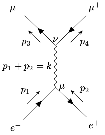
The corresponding expression is \begin{equation*} i\mathcal{T} = \bar{v}(p_2)(-e\gamma ^\mu ) \; iu(p_1) \; \left (-i \frac{\eta _{\mu \nu } -\frac{k_\mu k_\nu }{k^2}}{(k^2)}\right ) \bar{u}(p_3) \; (-e\gamma ^\nu ) \; i v(p_4), \end{equation*} with \(k= p_1+p_2 = p_3+p_4.\)
On-shell conditions. The external momenta are on-shell and the spinors \(u(p_1)\) etc. satisfy the Dirac equation, \begin{equation*} (ip_1 \cdot \gamma + m_e) u(p_1) = 0, \quad \quad \quad (-ip_4 \cdot \gamma + m_\mu ) v(p_4) = 0, \end{equation*} \begin{equation*} \bar{u}(p_3)(ip_3 \cdot \gamma + m_\mu )= 0,\quad \quad \quad \bar{v}(p_2)(-i p_2 \cdot \gamma + m_e) = 0. \end{equation*} This allows to write \begin{equation*} \begin{split} & i\bar v(p_2) \, \gamma ^\mu k_\mu \, u(p_1) = i\bar{v}(p_2) \, (p_1 \cdot \gamma + p_2 \cdot \gamma ) \, u(p_1) = \bar{v}(p_2) \, (-m_e + m_e) \, u(p_1) = 0, \\ & i\bar{u}(p_3) \, \gamma ^\nu k_\nu \, v(p_4) = i\bar{u}(p_3) \, (p_3 \cdot \gamma + p_4 \cdot \gamma) \, v(p_4) = \bar{u}(p_3) \, (-m_\mu + m_\mu ) \, v(p_4) = 0. \end{split} \end{equation*} These arguments show that the term \(\sim \) \(k_\mu k_\nu \) can be dropped. This is essentially a result of gauge invariance.
Complex conjugate and squared amplitudes. We are left with \begin{equation*} \mathcal{T} = \frac{e^2}{k^2} \bar{v}(p_2) \gamma ^\mu u(p_1) \, \bar{u}(p_3) \gamma _\mu v(p_4). \end{equation*} To calculate \(|\mathcal{T}|^2\) we also need \(\mathcal{T}^{*}\) which follows from hermitian conjugation \begin{equation*} \mathcal{T}^{*} = \frac{e^2}{k^2} v^\dagger (p_4) \gamma ^\dagger _\mu \bar{u}^\dagger (p_3) \; u^\dagger (p_1) \gamma ^{\mu \dagger } \bar{v}^\dagger (p_2). \end{equation*} Recall that \(\bar{u}(p) = u(p)^\dagger \beta \) with \(\beta = i\gamma ^0\). With the explicit representation \begin{equation*} \gamma ^\mu = \begin{pmatrix} & -i\bar{\sigma }^\mu \\ -i\sigma ^\mu & \end{pmatrix}, \end{equation*} it is also easy to prove \(\beta \gamma ^{\mu \dagger }\beta = -\gamma ^\mu \). By inserting \(\beta ^2 =\mathbb{1}\) at various places we find thus \begin{equation*} \mathcal{T}^{*} = \frac{e^2}{k^2} \bar{v}(p_4) \gamma _\mu u(p_3) \; \bar{u}(p_1)\gamma ^\mu v(p_2) \end{equation*} Putting together and using \(s=-k^2 = -(p_1+ p_2)^2\) we obtain \begin{equation*} |\mathcal{T}|^2 = \frac{e^4}{s^2} \bar{u}(p_1) \gamma ^\mu v(p_2) \; \bar{v}(p_2) \gamma ^\nu u(p_1) \; \bar{u}(p_3) \gamma _\nu v(p_1) \; \bar{v}(p_4) \gamma _\mu u(p_3). \end{equation*}
Spin sums and averages. To proceed further, we need to specify also the spins of the incoming and outgoing particles. The simplest case is the one of unpolarized particles so that we need to average the spins of the incoming electrons, and to sum over possible spins in the final state. Summing over the spins of the \(\mu ^{+}\) can be done as follows (exercise) \begin{equation*} \sum _{s=1}^2 v_s(p_4) \bar{v}_s(p_4) = -ip_4 \cdot \gamma -m_\mu , \end{equation*} and similarly for \(\mu ^{-}\) \begin{equation*} \sum _{s=1}^2 u_s(p_3) \bar{u}_s(p_3) = -ip_3 \cdot \gamma +m_\mu . \end{equation*} We can therefore write \begin{equation*} \bar{u}(p_3) \gamma _\nu v(p_4) \, \bar{v}(p_4) \gamma _\mu u(p_3) = \text{tr}\left \{(-ip_3 \cdot \gamma+m_\mu )\gamma _\nu (-ip_4 \cdot \gamma-m_\mu )\gamma _\mu \right \}. \end{equation*} Spins of the electron and positron must be averaged instead, \begin{equation*} \begin{split} \frac{1}{2}\sum _{s=1}^2 u(p_1) \bar{u}(p_1) & = \frac{1}{2}(-ip_1 \cdot \gamma+m_e),\\ \frac{1}{2}\sum _{s=1}^2 v(p_2) \bar{v}(p_2) & = \frac{1}{2}(-ip_2 \cdot \gamma-m_e). \end{split} \end{equation*} This leads to \begin{equation*} \frac{1}{4}\sum _{\text{spins}}|\mathcal{T}|^2 = \frac{e^4}{4s^2} \text{tr}\left \{(-ip_1 \cdot \gamma+m_e)\gamma ^\mu (-ip_2 \cdot \gamma-m_e) \gamma ^\nu \right \} \times \text{tr}\left \{(-ip_3 \cdot \gamma+m_\mu )\gamma _\nu (-i p_4 \cdot \gamma -m_\mu )\gamma _\mu \right \}. \end{equation*} In order to proceed further, we need to know how to evaluate traces of up to four gamma matrices.
Traces of gamma matrices. We need to understand how to evaluate traces of the form \(\text{tr}\{\gamma ^{\mu _1}\cdots \gamma ^{\mu _n}\}\) To work them out we can use \(\{\gamma ^\mu ,\gamma ^\nu \} = 2\eta ^{\mu \nu }\), \(\gamma _5^2 =\mathbb{1}\) and \(\{\gamma ^\mu ,\gamma _5\} = 0\). Also, \(\text{tr}\{\mathbb{1}\}=4\). First we prove that traces of an odd number of gamma matrices must vanish, \begin{equation*} \begin{split} \text{tr}\{\gamma ^{\mu _1}\cdots \gamma ^{\mu _n}\}&= \text{tr}\{\gamma _5^2\;\gamma ^{\mu _1} \gamma _5^2 \cdots \gamma _5^2 \gamma ^{\mu _n}\}\\ &=\text{tr}\{(\gamma _5 \gamma ^{\mu _1}\gamma _5)\cdots (\gamma _5 \gamma ^{\mu _1} \gamma _5)\}\\ &=\text{tr}\{(-\gamma _5^2\gamma ^\mu _1) \cdots (-\gamma _5^2\gamma ^{\mu _n})\}\\ &=(-1)^n \text{tr}\{\gamma ^{\mu _1}\cdots \gamma ^{\mu _n}\}. \end{split} \end{equation*} This implies what we claimed.
Now for even numbers \begin{equation*} \text{tr}\{\gamma ^\mu \gamma ^\nu \} = \text{tr}\{\gamma ^\nu \gamma ^\mu \} = \tfrac{1}{2} \text{tr}\{\gamma ^\mu \gamma ^\nu + \gamma ^\nu \gamma ^\mu \} = \eta ^{\mu \nu } \text{tr}\{\mathbb{1}\} = 4\eta ^{\mu \nu }. \end{equation*} From this it also follows that \begin{equation*} \text{tr}\{ p \cdot \gamma q \cdot \gamma\} = 4p \cdot q. \end{equation*} Now consider \(\text{tr}\{\gamma ^\mu \gamma ^\nu \gamma ^\rho \gamma ^\sigma \}.\) This idea is to commute \(\gamma ^\mu \) to the right using \(\{\gamma ^\mu ,\gamma ^\nu \} = 2\eta ^{\mu \nu }\). Thus \begin{equation*} \begin{split} \text{tr}\{\gamma ^\mu \gamma ^\nu \gamma ^\rho \gamma ^\sigma \} &= -\text{tr}\{\gamma ^\nu \gamma ^\mu \gamma ^\rho \gamma ^\sigma \} + 2\eta ^{\mu \nu }\;\text{tr}\{\gamma ^\rho \gamma ^\sigma \}\\ &= \text{tr}\{\gamma ^\nu \gamma ^\rho \gamma ^\mu \gamma ^\sigma \}-2\eta ^{\rho \mu } \text{tr}\{\gamma ^\nu \gamma ^\sigma \}+ 2\eta ^{\mu \nu }\;\text{tr}\{\gamma ^\rho \gamma ^\sigma \}\\ &= -\text{tr}\{\gamma ^\nu \gamma ^\rho \gamma ^\sigma \gamma ^\mu \} + 2\eta ^{\sigma \mu }\;\text{tr}\{\gamma ^\nu \gamma ^\rho \}- 2\eta ^{\rho \mu }\;\text{tr}\{\gamma ^\nu \gamma ^\sigma \}+ 2\eta ^{\mu \nu }\; \text{tr}\{\gamma ^\rho \gamma ^\sigma \}. \end{split} \end{equation*} But by the cyclic property of the trace \begin{equation*} \text{tr}\{\gamma ^\nu \gamma ^\rho \gamma ^\sigma \gamma ^\mu \} = \text{tr}\{\gamma ^\mu \gamma ^\nu \gamma ^\rho \gamma ^\sigma \} \end{equation*} which is also on the left hand side. Bringing it to the left and dividing by 2 gives \begin{equation*} \begin{split} \text{tr}\{\gamma ^\mu \gamma ^\nu \gamma ^\rho \gamma ^\sigma \} &= \eta ^{\sigma \mu }\;\text{tr}\{\gamma ^\nu \gamma ^\rho \}- \eta ^{\rho \mu }\;\text{tr}\{\gamma ^\nu \gamma ^\sigma \}+ \eta ^{\mu \nu }\text{tr}\{\gamma ^\rho \gamma ^\sigma \}\\ &= 4(\eta ^{\sigma \mu }\eta ^{\nu \rho }-\eta ^{\rho \mu }\eta ^{\nu \sigma }+ \eta ^{\mu \nu }\eta ^{\rho \sigma }). \end{split} \end{equation*} This is the result we were looking for. Clearly by using this trick we can in principle evaluate traces of an arbitrary number of gamma matrices.
Result so far. Coming back to \(e^{-}e^{+} \to \mu ^{-}\mu ^{+}\) we find \begin{equation*} \begin{split} \frac{1}{4} \sum _\text{spins} |\mathcal{T}|^2 = & \frac{4 e^4}{s^2}\left [-p_1^\mu p_2^\nu -p_1^\nu p_2^\mu + (p_1 \cdot p_2 - m_e^2) \eta ^{\mu \nu }\right ]\\ & \times \left [-(p_3)_\nu (p_4)_\mu -(p_3)_\mu (p_4)_\nu + (p_3 \cdot p_4 - m_\mu ^2) \eta ^{\mu \nu }\right ]\\ = & \frac{8 e^4}{s^2} \left [(p_1 \cdot p_4)(p_2 \cdot p_3)+(p_1 \cdot p_3)(p_2 \cdot p_4) -m_\mu ^2(p_1 \cdot p_2) -m_e^2(p_3 \cdot p_4) +2m_e^2 m_\mu ^2\right ] \end{split} \end{equation*} This looks already quite decent but it can be simplified even further in terms of Mandelstam variables.
The Mandelstam variables for a \(2\to 2\) process
are given by \begin{equation*} \begin{split} s &=-(p_1+p_2)^2 = -(p_3+p_4)^2, \\ t & = -(p_1-p_3)^2 = -(p_2-p_4)^2, \\ u &= -(p_1-p_4)^2 = -(p_2-p_3)^2. \end{split} \end{equation*} Together with the squares \(p_1^2\), \(p_2^2\), \(p_3^2\), \(p_4^2\), the Mandelstam variables can be used to express all Lorentz invariant bilinears in the momenta. Incoming and outgoing momenta are on-shell such that \(p_1^2 + m_1^2 =0\) etc. The sum of Mandelstam variables is \begin{equation*} s+t+u = -(p_1^2+ p_2^2+ p_3^2+ p_4^2) = m_1^2+ m_2^2+ m_3^2+m_4^2. \end{equation*} Using these variables for example through \begin{equation*} p_1 \cdot p_4 = -\frac{1}{2}\left [(p_1-p_4)^2-p_1^2-p_4^2\right ] = \frac{1}{2}\left [u-m_e^2+ m_\mu ^2\right ], \end{equation*} one finds for \( e^{-}e^{+} \to \mu ^{-}\mu ^{+}\) \begin{equation*} \frac{1}{4}\sum _\text{spins}|\mathcal{T}|^2 = \frac{2e^4}{s^2}\left [t^2+ u^2+ 4s(m_e^2+ m_\mu ^2)-2(m_e^2+ m_\mu ^2)^2\right ]. \end{equation*}
Differential cross section. From the squared matrix element we can calculate the differential cross section in the center of mass frame. For relativistic kinematics of \(2\to 2\) scattering and the normalization conventions we employ here one has in the center of mass frame \begin{equation*} \frac{d\sigma }{d\Omega } = \frac{1}{64\pi ^2 s}\frac{|\vec{p}_3|}{|\vec{p}_1|} \frac{1}{4} \sum _\text{spins}|\mathcal{T}|^2. \end{equation*} Let us express everything in terms of the energy \(E\) of the incoming particles and the angle \(\theta \) between the incoming \(e^{-}\) electron momenta and outgoing \(\mu ^{-}\) muon. \begin{equation*} \begin{split} |\vec{p}_1|=\sqrt{E^2 -m_e^2},\quad \quad \quad & s=4E^2, \\ |\vec{p}_3| = \sqrt{E^2 -m_\mu ^2},\quad \quad \quad & t=m_e^2+ m_\mu ^2-2E^2+2\vec{p}_1 \cdot \vec{p}_3, \\ \vec{p}_1 \cdot \vec{p}_3 = |\vec{p}_1||\vec{p}_3|\cos \theta , \quad \quad \quad & u = m_e^2 + m_\mu ^2 - 2E^2 -2\vec{p}_1 \cdot \vec{p}_3. \end{split} \end{equation*} With these relations we can express \(\frac{d\sigma }{d\Omega }\) in terms of \(E\) and \(\theta \) only.
Ultrarelativistic limit. Let us concentrate on the ultrarelativistic limit \(E\gg m_e, m_\mu \) so that we can set \(m_e = m_\mu = 0\). One has then \(|\vec{p}_1|=|\vec{p}_3|\) and \begin{equation*} t^2 + u^2 = 8E^4(1+ \cos ^2\theta ), \quad \quad \quad \frac{2(t^2+ u^2)}{s^2}= 1+ \cos ^2 \theta , \end{equation*} which leads to \begin{equation*} \frac{d\sigma }{d\Omega } = \frac{e^4}{64\pi ^2 s}(1+\cos ^2 \theta ) = \frac{\alpha ^2}{4s}(1+\cos ^2 \theta ). \end{equation*} In the last equation we used \(\alpha = e^2/ (4\pi )\).