Quantum field theory 1, lecture 25
10.7 Higgs/Yukawa theory
In the following two lectures we will discuss a quantum field theoretic model that extends somewhat beyond quantum electrodynamics. We add to the theory a neutral massive scalar field that couples to the fermions through a Yukawa interaction. One may see that additional massive scalar particle as an analog of the Higgs boson, even though our model reflects only a few of the properties of the real electroweak standard model.
We discuss the model as a further example for an interesting quantum field theory and because we can nicely study there decay processes.
- A massive Higgs boson can decay into two fermions through the Yukawa interaction. This is a tree level process and rather easy to calculate.
- Interestingly a neutral and massive Higgs boson can also decay into two photons. This process is not allowed at tree level (because the Higgs boson is neutral), but it is induced by loop diagrams. This will be the first loop diagram we will calculate in detail.
In the second part of the lecture course loop diagrams and their physical consequences will be studied in much more detail. For the Higgs decay into photons we do not need renormalization yet, which simplifies the discussion. Nevertheless there will be some new elements to be discussed.
Action for Higgs/Yukawa theory and fermion mass. Let us consider the following extension of QED by a neutral scalar field (with \(m=gv\)) \begin{equation*} \begin{split} S[\bar{\psi },\psi , A, \phi ] = & \int _x {\Big\{ } -i\bar{\psi } \gamma ^\mu \left (\partial _\mu - ieA_\mu \right )\psi - im\bar{\psi } \psi \\ & -\frac{1}{4} F^{\mu \nu }F_{\mu \nu } -\frac{1}{2} \phi \left (-\partial _\mu \partial ^\mu + M^2 \right )\phi - i g \phi \bar{\psi }\psi {\Big \}}. \end{split}\end{equation*} Note that a constant (homogeneous) scalar field \(\phi \) modifies the fermion mass according to \begin{equation*} m_\text{eff} = m+ g\phi = g(v+\phi ) \end{equation*} In fact, one can understand the massses of elementary fermions (leptons and quarks) in the standard model of elementary particle physics as being due to such a scalar field expectation value for the Higgs field.
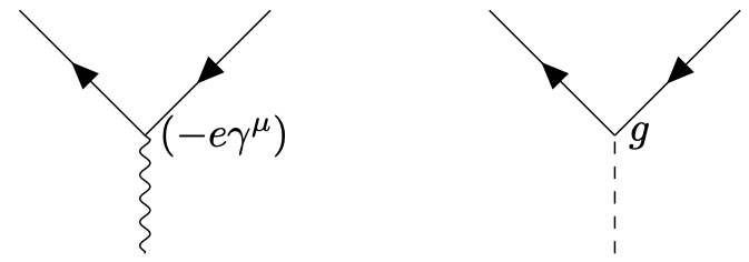
Propagators and vertices. In the theory above we have now different propagators
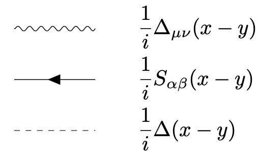
with scalar propagator \begin{equation*} \Delta (x-y) = \int _p e^{ip(x-y)} \frac{1}{p^2 + M^2}. \end{equation*} The vertices are
10.8 Higgs decay into fermions
Higgs decay to fermions. Let us discuss first the process \(\phi \to f^{-}f^{+}.\) The fermions could be leptons (\(e\), \(\mu \), \(\tau \)) or quarks (\(u\), \(d\), \(s\), \(c\), \(b\), \(t\)). The Feynman diagram for the decay is simply
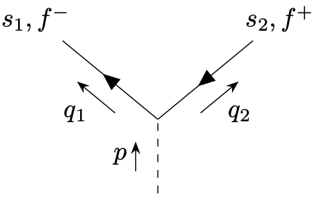
According to the Feynman rules we obtain \begin{equation*} i\mathcal{T} = g \; \bar{u}_{s_1}(q_1) iv_{s_2}(q_2),\quad \quad \quad \mathcal{T}^* = g \; \bar{v}_{s_2}(q_2) u_{s_1}(q_1). \end{equation*} For the absolute square one finds \begin{equation*} |\mathcal{T}|^2 = g^2 \, \bar{u}_{s_1}(q_1) v_{s_2}(q_2) \, \bar{v}_{s_2}(q_2) u_{s_1}(q_1). \end{equation*}
Spin sums and Dirac traces. We will assume that the final spins are not observed and sum them \begin{equation*} \sum _\text{spins} |\mathcal{T}|^2 = g^2 \; \text{tr}\left \{(-iq_2 \cdot \gamma - m)(-iq_1 \cdot \gamma + m) \right \} \end{equation*} We used here again the spin sum formula \begin{equation*} \sum _s v_s(p) \bar{v}_s(p) = -ip \cdot \gamma-m,\quad \quad \quad \sum _s u_s(p) \bar{u}_s(p) = -ip \cdot \gamma+m. \end{equation*} Performing also the Dirac traces gives \begin{equation*} \sum _{\text{spins}} |\mathcal{T}|^2 = g^2 \left (-4 q_1 \cdot q_2 - 4m^2 \right ). \end{equation*}
Kinematics in the Higgs boson rest frame. Let us now go into the rest frame of the decaying particle where \begin{equation*} p=(M,0,0,0), \quad \quad \quad q_1 = \left (\tfrac{M}{2}, \vec{q} \right ),\quad \quad \quad q_2= \left (\tfrac{M}{2}, -\vec{q} \right ), \end{equation*} with \begin{equation*} \vec{q}^2 = -m^2 + \tfrac{M^2}{4}, \quad \quad q_1 \cdot q_2= -\frac{M^2}{4} - \vec{q}^2 = -\frac{M^2}{m^2}, \end{equation*} and \begin{equation*} \sum _{\text{spins}}|\mathcal{T}|^2 = 2 \, g^2 M^2 \left (1-4\frac{m^2}{M^2}\right ). \end{equation*} Note that the decay is kinematically possible only for \(M>2m\) so that the bracket is always positive.
Decay rate. For the particle decay rate we get \begin{equation*} \frac{d \Gamma }{d\Omega } = \frac{|\vec{q}_1|}{32 \pi ^2 M^2} \sum _{\text{spins}}|\mathcal{T}|^2 =\frac{g^2 M}{32 \pi ^2}\left (1-4\frac{m^2}{M^2}\right )^{3/2}. \end{equation*} Because this is independent of the solid angle \(\Omega \) one can easily integrate to obtain the decay rate \begin{equation*} \Gamma = \frac{g^2 M}{8\pi }\left (1-4\frac{m^2}{M^2}\right )^{3/2}. \end{equation*}
Dependence on fermion mass. If the scalar boson \(\phi \) is the Higgs boson, the Yukawa coupling is in fact proportional to the fermion mass \(m\), \begin{equation*} g = \frac{m}{V}. \end{equation*} One has then \begin{equation*} \Gamma = \frac{M^3}{32 \pi v^2} \, f\left (\frac{2m}{M} \right ) \end{equation*} where \begin{equation*} f(x) = x^2 (1-x^2)^{3/2} \end{equation*}
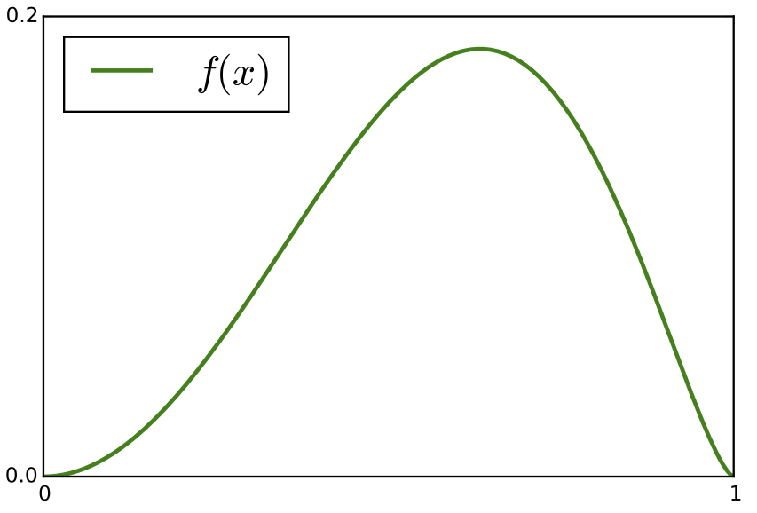
Decay into light fermions is suppressed because of small coupling while decay into very heavy fermions is suppressed by small phase space or even kinematically excluded for \(2m > M\).
For Higgs boson mass of \(M= 125\) GeV the largest decay rate to fermions is to \(b\bar{b}\) (bottom quark and anti-quark). This corresponds to \(m = 4.18\) GeV. The top quark would have larger coupling but is in fact too massive (\(m = 172\) GeV). (The lepton with largest mass is the tauon \(\tau \) with \(m = 1.78\) GeV.)
10.9 Higgs decay into photons
Higgs decay into photons. A Higgs particle can also decay into photons and this is in fact how it was discovered. How is this possible? If we try to write down a diagram in the theory introduced above we realize that there is no tree diagram. However, there are loop diagrams!
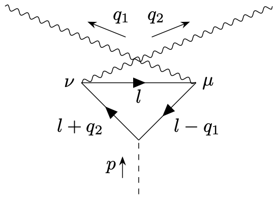
Consider the diagrams
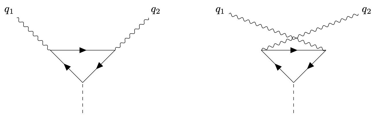
These terms arise from the expansion of the partition function if the fermion propagator appears \(3\) times and there are \(2\) fermion-photon and one fermion-scalar vertices.
Signs in fermion loops. Schematically, the vertices are derivatives \begin{equation*} \left [(-e\gamma ^\mu ) \left (\frac{1}{i} \frac{\delta }{\delta J^\mu }\right )\left (i \frac{\delta }{\delta \eta }\right ) \left (\frac{1}{i} \frac{\delta }{\delta \bar{\eta }}\right )\right ] \quad \quad \quad \text{or} \quad \quad \quad \left [g \left (\frac{1}{i}\frac{\delta }{\delta J}\right )\left (i\frac{\delta }{\delta \eta }\right )\left (\frac{1}{i}\frac{\delta }{\bar{\eta }}\right )\right ] \end{equation*} and they act here on a chain like \begin{equation*} \left [(i\bar{\eta })\left (\frac{1}{i}S\right )(i\eta )\right ]\left [(i\bar{\eta }\left (\frac{1}{i}S \right )(i\eta )\right ]\left [(i\bar{\eta })\left (\frac{1}{i}S \right )(i\eta )\right ]. \end{equation*} Note that the derivative with respect to \(\bar{\eta }\) can be commuted through the square brackets and acts on \(\bar{\eta }\) from the left. Factors \(1/i\) and \(i\) cancel. The derivative with respect to \(\eta \) receives an additional minus sign from commuting and this cancels against \(i^2\). In this way the vertices can connect the elements of the chain. However, for a closed loop also the beginning and end of the chain must be connected. To make this work, one can first bring the \((i\eta )\) from the end of the chain to its beginning. This leads to one additional minus sign from anti-commuting Grassmann fields. This shows that closed fermion lines have one more minus sign.
Position space representation. In position space and including sources, the first diagram is
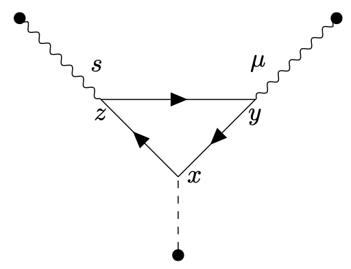
\begin{equation*} \begin{split} & g(-1) \int _{x,y,z} \text{tr}\left \{ \left [\frac{1}{i}S(x-y) \right ](-e\gamma ^\mu ) \left [\frac{1}{i}S(y-z) \right ] (-e\gamma ^\nu ) \left [\frac{1}{i}S(z-x) \right ]\right \}\\ & \times \int _{u,v,w} \left [\frac{1}{i}\Delta _{\mu \alpha }(y-u) \right ] (iJ^\alpha (u)\left [\frac{1}{i}\Delta _{\nu \beta }(z-v) \right ] (iJ^\beta (v) \left [\frac{1}{i}\Delta (x-w) \right ](iJ(w)) \end{split} \end{equation*} The trace is for the Dirac matrix indices.
Momentum space representation for first diagram. If one translates this now to momentum space and considers the amputated diagram for an S-matrix element, one finds that momentum conservation constrains momenta only up to one free integration momentum or loop momentum. In fact, more generally, there is one integration momentum for every closed loop. The first diagram is then
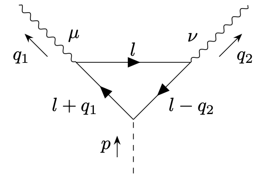
\begin{equation*} \begin{split} &(-1)ge^2\;\epsilon ^{*}_\mu (q_1) \epsilon ^{*}_\nu (q_2) \int _l \frac{1}{[l+q_1)^2 + m^2 -i\epsilon ][l^2 + m^2 -i\epsilon ][l-q_2)^2 + m^2 + i\epsilon ]}\\ & \times \text{tr} \left \{ \left [-i(l \cdot \gamma+q_1 \cdot \gamma)+m \right ] \gamma ^\mu \left [-il \cdot \gamma+m \right ] \gamma ^nu \left [-i(l \cdot \gamma-q_2 \cdot \gamma)+m \right ] \right \} \end{split} \end{equation*} Here we use here the abbreviation \begin{equation*} \int _l = \int \frac{d^4 l}{(2\pi )^4}. \end{equation*}
Momentum space representation for second diagram. For the second diagram we can write
\begin{equation*} (-1)ge^2\;\epsilon ^{*}_\mu (q_1) \;\epsilon ^{*}_\nu (q_2) \int _l \ldots \end{equation*} where the integrand is the same up to the interchange \(q_1 \leftrightarrow q_2\) and \(\mu \leftrightarrow \nu \). We can therefore concentrate on evaluating the first diagram.
Analytic continuation and Dirac traces. The Feynman \(i\epsilon \) terms allow to perform a Wick rotation to Euclidean space \(l^0 = i\tilde{l}^0_E\) so that \(l^2\) is then positive. Let us count powers of \(l\). First, in the Dirac trace we have terms with up to 5 gamma matrices. However, only traces of an even number of gamma matrices are non-zero.
With a bit of algebra one finds for the Dirac trace \begin{equation*} \begin{split} & \text{tr} \left \{ \left [-i (l \cdot \gamma+q_1 \cdot \gamma)+m \right ] \gamma ^\mu \left [-il \cdot \gamma+m \right ] \gamma ^\nu \left [-i(l \cdot \gamma-q_2 \cdot \gamma)+m \right ] \right \}\\ & = -m \;\text{tr}\left \{(l \cdot \gamma+q_1 \cdot \gamma)\gamma ^\mu l \cdot \gamma\gamma ^\nu + (l \cdot \gamma+q_1 \cdot \gamma) \gamma ^\mu \gamma ^\nu (l \cdot \gamma-q_2 \cdot \gamma)+ \gamma ^\mu l \cdot \gamma\gamma ^\nu (l \cdot \gamma-q_2 \cdot \gamma) \right \} \\ & \;\;\;\;+m^3\;\text{tr} \left \{\gamma ^\mu \gamma ^\nu \right \}\\ &=-4m{\Big [} (l+q_1)^\mu l^\nu + (l+q_1)^\nu l^\mu -(l+q_1) \cdot l\;\eta ^{\mu \nu }\\ & \quad \quad \quad + (l+q_1)^\mu (l-q_2)^\nu + (l+q_1) \cdot (l-q_2) \eta ^{\mu \nu } -(l+q_1)^\nu (l-q_2)^\mu \\ &\quad \quad \quad + l^\mu (l-q_2)^\nu + (l-q_2)^\mu l^\nu -\eta ^{\mu \nu } l \cdot (l-q_2){\Big ]} + 4 \eta ^{\mu \nu } m^3\\ &= -4m \left [4 l^\mu l^\nu -l^2 \eta ^{\mu \nu } -l^2 \eta ^{\mu \nu } + 2q^\mu _1 l^\nu -2q^\nu _2 l^\mu -q^\mu _1 q^\nu _2 + q^\nu _1 q^\mu _2 -(q_1 \cdot q_2) \eta ^{\mu \nu } \right ] + 4\eta ^{\mu \nu } m^3. \end{split} \end{equation*}