
Quantum field theory 1, lecture 24
Electron-Muon Scattering. We can also consider the scattering process \(e^{-} \mu ^{-} \to e^{-}\mu ^{-}\),
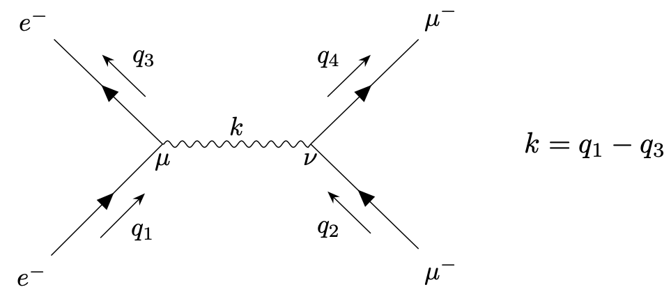
\begin{equation*} i \mathcal{T} = \bar{u}(q_3) (-e\gamma ^\mu ) iu(q_1) \left (-i\frac{\eta _{\mu \nu } -\frac{k_\mu k_\nu }{k^2}}{k^2}\right )\bar{u}(q_4)(-e\gamma ^\nu ) iu(q_2). \end{equation*} By a similar argument as before the term \(\sim k_\mu k_\nu \) drops out, \begin{equation*} \mathcal{T} = \frac{e^2}{(q_1-q_3)^2} \bar{u}(q_3) \gamma ^\mu u(q_1) \bar{u}(q_4) \gamma _\mu u(q_2)\quad \quad \quad (e^{-}\mu ^{-} \to e^{-}\mu ^{-}). \end{equation*}
Comparison to electron to muon scattering. Compare this to what we have found for \(e^{-} e^{+} \to \mu ^{-}\mu ^{+}\) \begin{equation*} \mathcal{T} = \frac{e^2}{(p_1+p_2)^2} \bar{v}(p_2) \gamma ^\mu u(p_1) \bar{u}(p_3) \gamma _\mu v(p_4), \end{equation*} where the conventions were according to
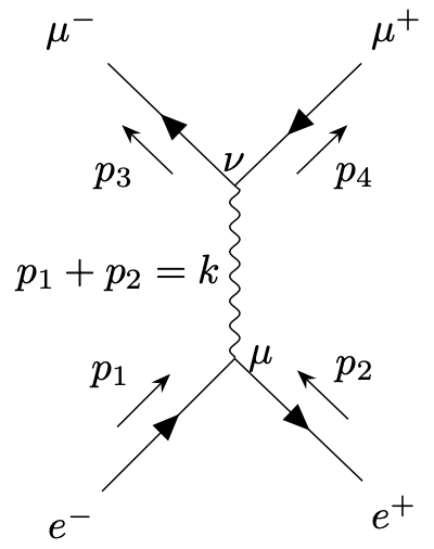
There is a close relation and the expressions agree if we put \begin{equation*} \begin{split} q_1 = +p_1, \quad \quad \quad & u(q_1) = u(p_1), \\ q_2 = -p_4, \quad \quad \quad & u(q_2) = u(-p_4) \to v(p_4), \\ q_3 = -p_2, \quad \quad \quad & \bar{u}(q_3) = \bar{u}(-p_2) \to \bar{v}(p_2), \\ q_4 = +p_3, \quad \quad \quad & \bar{u}(q_4) = \bar{u}(p_3). \end{split} \end{equation*}
Crossing symmetry. Recall that \begin{equation*} (ip \cdot \gamma+m)\;u(p) = 0 \quad \quad \quad \text{but} \quad \quad \quad (-ip \cdot \gamma+ m)\;v(p) = 0. \end{equation*} However one sign arises from the spin sums \begin{equation*} \begin{split} \sum _{s=1}^2 \; u_s(p)\bar{u}_s(p) & =-ip \cdot \gamma+m, \\ \sum _{s=1}^2 \; v_s(p)\;\bar{v}_s(p) & = -ip \cdot \gamma-m = -\sum _s u_s(-p)\;\bar{u}_s(-p). \end{split} \end{equation*} Because it appears twice, the additional sign cancels for \(|\mathcal{T}|^2\) after spin averaging and one finds indeed the same result as for \(e^{-}e^{+} \to \mu ^{-}\mu ^{+}\) but with \begin{equation*} \begin{split} s_q = & -(q_1+q_2)^2 = -(p_1-p_4)^2 = u_p, \\ t_q = & -(q_1 -q_3)^2 = -(p_1+p_2)^2 = s_p,\\ u_q = & -(q_1 -q_4)^2 = -(p_1 -p_3)^2 =t_p. \end{split} \end{equation*} We can take what we had calculated but must change the role of \(s\), \(t \)and \(u\) ! This is an example of crossing symmetries.
Electron-muon scattering in the massless limit. Recall that we found for \(e^{-}e^{+} \to \mu ^{-}\mu ^{+}\) in the massless limit \(m_e = m_\mu = 0\) simply \begin{equation*} \frac{1}{4}\sum _\text{spins} |\mathcal{T}|^2 = \frac{2e^4}{s^2} \left [t^2+u^2 \right ]. \end{equation*} For \(e^{-}\mu ^{-} \to e^{-}\mu ^{-}\) we find after the replacements \(u \to s\), \(s\to t\), \(t \to u\), \begin{equation*} \frac{1}{4} \sum _\text{spins}|\mathcal{T}|^2=\frac{2e^4}{t^2}\left [u^2+ s^2\right ]. \end{equation*}
More on Mandelstam variables. To get a better feeling for \(s\), \(t\) and \(u\), let us evaluate them in the center of mass frame for a situation where all particles have mass \(m\).
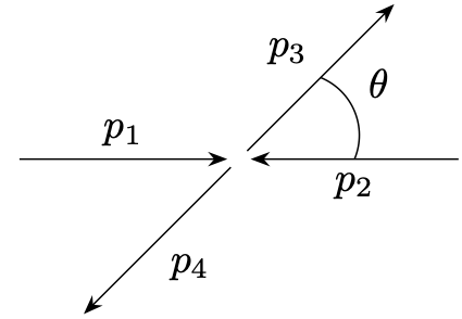
\begin{equation*} \begin{split} p_1^\mu & =(E,\vec{p}),\quad \quad p_2^\mu =(E,-\vec{p}), \\ p_3^\mu & =(E,\vec{p}'), \quad \quad p_4^\mu =(E, -\vec{p}'). \\ \end{split} \end{equation*} While \(s\) measures the center of mass energy, \(t\) is a momentum transfer that vanishes in the soft limit \(\vec{p}^2 \to 0\) and in the colinear limit \(\theta \to 0.\) Similarly, \(u\) vanishes for \(\vec{p}^2 \to 0\) and for backward scattering \(\theta \to \pi .\)
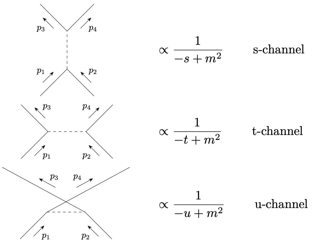
\(s\)-, \(t\)- and \(u\)-channels. One speaks of interactions in different channels for tree diagrams of the following generic types,
Electron-muon scattering. For the cross section we find for \(e^{-}\mu ^{-} \to e^{-}\mu ^{-}\) in the massless limit \begin{equation*} \frac{d\sigma }{d\Omega } = \frac{1}{64\pi ^2 s} \frac{1}{4} \sum _{\rm spins} |\mathcal{T}|^2 = \frac{\alpha ^2[4+(1+\cos \theta )^2]}{2s(1-\cos \theta )^2} \end{equation*} This diverges in the colinear limit \(\theta \to 0\) as we had already seen for Yukawa theory in the limit where the exchange particle becomes massless.
Note that by the definition \(s \geq 0\) while \(u\) and \(t\) can have either sign. Replacements of the type used for crossing symmetry are in this sense always to be understood as analytic continuation.
10.6 Relativistic scattering and decay kinematics
Covariant normalization of asymptotic states. For non-relativistic physics this we have used a normalization of single particle states in the asymptotic incoming and out-going regimes such that \begin{equation*} \langle \vec{p}|\vec{q}\rangle = (2\pi )^3 \delta ^{(3)}(\vec{p}-\vec{q}). \end{equation*} For relativistic physics this has the drawback that it is not Lorentz invariant. To see this let us consider a boost in \(z\)-direction \begin{equation*} \begin{split} E^\prime =& \gamma (E+\beta p^3), \\ p^{1\prime } = & p^{1}, \\ p^{2\prime } = & p^2, \\ p^{3\prime } = & \gamma (p^3+\beta E). \end{split} \end{equation*} Using the identity \begin{equation*} \delta \left (f(x) - f(x_0) \right ) = \frac{1}{|f'(x_0)|}\delta (x-x_0), \end{equation*} one finds \begin{equation*} \begin{split} \delta ^{(3)}(\vec{p}-\vec{q}) &= \delta ^{(3)}(\vec{p}^\prime -\vec{q}^\prime ) \frac{dp^{3\prime }}{dp^3} = \delta ^{(3)}(\vec{p}-\vec{q}) \gamma \left (1+\beta \frac{dE}{dp^3} \right )\\ &= \delta ^{(3)}(\vec{p}'-\vec{q}') \frac{1}{E}\gamma \left (E+\beta p^3 \right )\\ &= \frac{E^\prime }{E} \delta ^{(3)} (\vec{p}^\prime - \vec{q}^\prime ). \end{split} \end{equation*} This shows, however, that \(E\;\delta ^{(3)} (\vec{p}-\vec{q})\) is in fact Lorentz invariant.
This motivates to change the normalization such that \begin{equation*} |p; \text{in}\rangle = \sqrt{2E_p} a^\dagger _{\vec{p}}(-\infty ) |0\rangle = \sqrt{2E_{\vec{p}}} \, |\vec{p}; \text{in} \rangle . \end{equation*} Note the subtle difference in notation between \(|p; \text{in}\rangle \) (relativistic normalization) and \(|\vec p; \text{in}\rangle \) (non-relativistic normalization). This implies for example \begin{equation*} \langle p; \text{in}| q; \text{in} \rangle = 2E_p (2\pi )^3 \delta ^{(3)}(\vec{p}-\vec{q}). \end{equation*} With this normalization we must divide by \(2E_p\) at the same places. In particular the completeness relation for single particle incoming states is \begin{equation*} \mathbb{1}_{1-\text{particle}} = \int \frac{d^3p}{(2\pi )^3} \frac{1}{2E_{\vec{p}}}|p;\text{in}\rangle \langle p; \text{in}|. \end{equation*} In fact, what appears here is a Lorentz invariant momentum measure. To see this consider \begin{equation*} \int \frac{d^4 p}{(2\pi )^4}\;(2\pi )\;\delta (p^2+m^2)\;\theta (p^0) = \int \frac{d^3p}{(2\pi )^3} \frac{1}{2E_{\vec{p}}}. \end{equation*} The left hand side is explicitly Lorentz invariant and so is the right hand side.
Covariantly normalized S-matrix. We can use the covariant normalization of states also in the definition of S-matrix elements. The general definition is as before \begin{equation*} S_{\beta \alpha } = \langle \beta ; \text{out}| \alpha ; \text{in}\rangle = \delta _{\beta \alpha }+ i \, \mathcal{T}_{\beta \alpha }(2\pi )^4 \delta ^{(4)}(p^\text{in}-p^\text{out}). \end{equation*} But now we take elements with relativistic normalization, e.g. for \(2 \to 2\) scattering \begin{equation*} S_{q_1q_2, p_1p_2} = \langle q_1,q_2; \text{out}| p_1,p_2 ; \text{in}\rangle . \end{equation*} We can calculate these matrix elements as before using the LSZ reduction formula to replace \(\sqrt{2E_p} a^\dagger _{\vec{p}}(-\infty )\) by fields. For example, for relativistic scalar fields \begin{equation*} \sqrt{2 E_{\vec{p}}}\; a^\dagger _{\vec{p}}(-\infty ) = \sqrt{2E_{\vec{p}}} \; a^\dagger _{\vec p}(\infty ) + i\left [-(p^0)^2+ \vec{p}^2 + m^2\right ] \phi ^{*}(p). \end{equation*} This allows to calculate S-matrix elements through correlation functions.
Cross sections for \(2\to n\) scattering. Let us now generalize our discussion of \(2 \to 2\) scattering of non-relativistic particles to a scattering \(2 \to n\) of relativistic particles. The transition probability is as before \begin{equation*} P = \frac{|\langle \beta ; \text{out}| \alpha ; \text{in}\rangle |^2}{\langle \beta ; \text{out}| \beta ;\text{out}\rangle \langle \alpha ; \text{in}| \alpha ; \text{in}\rangle }. \end{equation*} Rewriting the numerator in terms of \(\mathcal{T}_{\beta \alpha }\) and going over to the transition rate we obtain as before \begin{equation} \dot{P} = \frac{V (2\pi )^4 \delta ^{(4)}(p^\text{out}-p^\text{in})|\mathcal{T}|^2}{\langle \beta ; \text{out}| \beta ;\text{out}\rangle \langle \alpha ; \text{in}| \alpha ; \text{in}\rangle }. \label{eq:PDot} \end{equation} But now states are normalized in a covariant way \begin{equation*} \begin{split} \langle p| p \rangle &= \lim _{q \to p} \langle p|q \rangle \\ &= \lim _{q \to p} 2E_p (2\pi )^3 \delta ^{(3)}(\vec{p}-\vec{q})\\ &= 2E_p (2\pi )^3 \delta ^{(3)}(0)\\ &= 2E_p V \end{split} \end{equation*} One has thus for the incoming state of two particles \begin{equation*} \langle \alpha ; \text{in}| \alpha ; \text{in}\rangle = 4E_1 E_2 V^2. \end{equation*} For the outgoing state of \(n\) particles one has instead \begin{equation*} \langle \beta ; \text{out}| \beta ; \text{out}\rangle = \prod _{j=1}^n \{2q^0_j V\}. \end{equation*} The product goes over final state particles which have the four-momentum \(q_j^n\). So, far we have thus \begin{equation*} \dot{P} = \frac{V\;(2\pi )^4\;\delta ^{(4)}(p^\text{in} - p^\text{out})|\mathcal{T}|^2}{4E_1 E_2 V^2\; \prod _{j=1}^n \{2q_j^0 V\} }. \end{equation*}
Lorentz invariant phase space. To count final state momenta appropriately we could go back to finite volume and then take the continuum limit. This leads to an additional factor \begin{equation*} \sum _{\vec{n}_j} \to V\;\int \frac{d^3 q}{(2\pi )^3} \end{equation*} for each final state particle. The transition rate becomes \begin{equation*} \dot{P} = \frac{|\mathcal{T}|^2}{4E_1 E_2 V} \left [(2\pi )^4\;\delta ^{(4)}{\Big (}p^\text{in}-\sum _j q_j{\Big )} \prod _{j=1}^n \left \{\frac{d^3 q_j}{(2\pi )^3 2q^0_j}\right \}\right ] \end{equation*} The expression in square brackets is known as the Lorentz-invariant phase space measure (sometimes ”LIPS”).
Flux and differential cross section. To go from there to a differential cross section we need to divide by a flux of particles. There is one particle per volume \(V\) with velocity \(v=v_1 - v_2\), so the flux is \begin{equation*} \mathcal{F} = \frac{|v|}{V} = \frac{|v_1-v_2|}{V} = \frac{\left |\frac{p_1^3}{p_1^0}-\frac{p_2^3}{p_2^0}\right |}{V}. \end{equation*} In the last equality we chose the beam axis to coincide with the \(z\)-axis. For the differential cross section we obtain \begin{equation*} d\sigma = \frac{|\mathcal{T}|^2}{4E_1 E_2 |v_1-v_2|}\; [\text{LIPS}]. \end{equation*} The expression in the prefactor can be rewritten like \begin{equation*} \frac{1}{E_1 E_2 |v_1- v_2|} = \frac{1}{p_1^0 p_2^0 \left |\frac{p_1^3}{p_1^0}-\frac{p_2^3}{p_2^0}\right |} = \frac{1}{| p_2^0 p_1^3 - p_1^0 p_2^3 |} = \frac{1}{|\epsilon _{\mu x y \nu } p_2^\mu p_1^\nu |}. \end{equation*} This is not Lorentz invariant in general but invariant under boosts in the \(z\)-direction. In fact it transforms as a two-dimensional area element as it should.
Differential cross section in the centre of mass frame. In the center of mass frame one has \(p_2^3 = -p_1^3 = \pm |\vec{p}_1|\) and \begin{equation*} \frac{1}{|p_2^0 p_1^3 -p_1^0 p_2^0|} = \frac{1}{|\vec{p}_1|(p_1^0 + p_2^0)} = \frac{1}{|\vec{p}_1|_\text{COM}\sqrt{s}} \end{equation*} This leads finally to the result for the differential cross section \begin{equation*} d\sigma = \frac{|\tau |^2}{4 |\vec{p}_1|_{\text{COM}}\sqrt{s}} \left [ (2\pi )^4 \delta ^{(4)}{\Big (}p^\text{in}-\sum _j q_j{\Big )} \prod _{j=1}^n \left \{\frac{d^3 q_j}{(2\pi )^3 2q_j^0}\right \}\right ]. \end{equation*}
\(2 \to 2\)scattering. For the case of \(n=2\) one can write the Lorentz invariant differential phase space element in the center of mass frame (exercise) \begin{equation*} \left [(2\pi )^4 \; \delta ^{(4)} (p^{\text{in}} -q_1 -q_2) \frac{d^3 q_1}{(2\pi )^3 2q_1^0}\; \frac{d^3 q_2}{(2\pi )^3 q_2^0}\right ] = \frac{|\vec{q}_1|}{16 \pi ^2 \sqrt{s}}d\Omega \end{equation*} such that \begin{equation*} \frac{d\sigma }{d\Omega } = \frac{1}{64\pi ^2 s} \frac{|\vec{q}_1|}{|\vec{p}_1|} |\mathcal{T}|^2. \end{equation*}
Decay rate. Let us now consider the decay rate of a single particle, i. e. a process \(1 \to n\). We can still use equation \eqref{eq:PDot}, but now the initial state is normalized like \begin{equation*} \langle \alpha ; \text{in}|\alpha ; \text{in}\rangle = 2E_1 V. \end{equation*} We find then for the differential transition or decay rate \(d\Gamma = \dot{P}\) \begin{equation*} d\Gamma = \frac{|\mathcal{T}|^2}{2E_1}\left [(2\pi )^4 \delta ^{(4)}{\Big (}p^{\text{in}}-\sum _j q_j{\Big )} \prod _{j=1}^n \left \{\frac{d^3 q_j}{(2\pi )^3 2q_j^0}\right \}\right ] \end{equation*} In the center of mass frame one has \(E_1 = m_1\). For the special case of \(1\to 2\) decay one finds in the center of mass frame or rest frame of the initial particle \begin{equation*} d\Gamma = \frac{|\mathcal{T}|^2 |\vec{q}_1|}{32 \pi ^2 m_1^2} d\Omega . \end{equation*}